ICSE X Class Maths

ICSE X Class Maths Concept designed by the ‘Basics in Maths’ team. These notes to do help the ICSE 10^th class Maths students fall in love with mathematics and overcome their fear.

These notes cover all the topics covered in the ICSE 10^th class Maths syllabus and include plenty of formulae and concept to help you solve all the types of 10^th class Mathematics problems asked in the ICSE board and entrance examinations.

 1. Goods and Service Tax

Two types of taxes in the Indian Government:

1.Direct taxes: –

These are the taxes paid by an organisation or individual directly to the government. These include Income tax, Capital gain tax and Corporate tax.

2.Indirect taxes: –

These are the taxes on goods and services paid by the customer, collected by an individual or an organisation and deposited with the Government. Earlier there were several indirect taxes levied by the central and state Governments.

Goods and Service Tax (GST):

GST is a comprehensive indirect tax for the whole nation. It makes India one unified common market.

 Registration under GST:

Any individual or organisation that has an annual turnover of more than ₹ 20 lakh is to be registered under GST.

Input and Output GST:

For any individual or organisation, the GST paid on purchases is called the ‘Input GST’ and the GST collection on sale of goods is called the ‘Output GST’. The input GST is set off against the output GST and the difference between the two is payable in the Government account.

One currency one tax:

There is a uniform GST rate on any particular goods or services across all states and Union Territories of India. This is called ‘One currency one tax’.

Note: Assam was the first state to implement GST and Jammu & Kashmir was the last.

GST rate slabs:

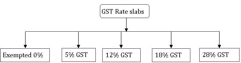
However, the tax on gold is kept at 3% and on rough precious and semi-precious is kept at 0.25%.

The multitier GST tax rate system in India has been developed keeping in mind that essential commodities should be taxed less than luxury goods.

Benefits of GST for Traders:

• Simple tax system.

• Elimination of multiplicity of taxes.

• Development of a common market nation-wide.

• Reduction of cascading effect.

• Lower taxes result in the reduction of costs making in the domestic market.

Benefits of GST for Consumers:

• Single and transparent System.

• Elimination of cascading effect has resulted in the reduction in the costs of goods and services.

• Increase in purchasing power and savings.

Benefits of GST for Traders:

• Single tax system, simple and easy to administer.

• Higher revenue efficiency.

• Better control on leakage and tax evasion.

Types of GST in India

Central GST (CGST): For any intrastate supply half of the GST collected as the output GST is deposited with the Central Governments as CGST.

State GST or Union Territory GST (SGST/UGST): For any local supply (supply with in the same state or Union Territory) half of the GST is deposited with the respective state or Union Territory Government as the beneficiary. This is called SGST/UGST.

Integrated GST (IGST): The GST levied on the supply of goods or services in the case of interstate trade within India or in the case of exports/imports is known as IGST.

Reverse charge Mechanism:

There are cases where the chargeability gets reversed, that is the receiver becomes liable to pay the tax and deposit it to the Government Account.

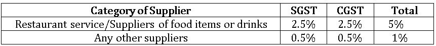
Composition shame:

The composition is meant for small dealers and service providers with an annual turnover less than ₹ 1.5 crores and also for Restaurant service providers. Under this scheme the rates of GST are:

Input Tax Credit (ITC)    

When a dealer sells his goods, he charges the output GST from his customer which he has to deposit in the government account, but in running his business he had paid input GST on the goods he had availed. This input GST, he utilizes as Input Tax credit and deposits the exes amount of output GST with the Government.

Input Tax credit is a provision of reducing the GST already paid on inputs in order to avoid the cascading of taxes.

GST payable = Output GST – ITC

Claiming ITC: A dealer registered under GST can claim ITC only if:

• He possesses the tax invoice.
• He has received the said goods/services
• He has filed the returns.
• The tax paid by him has been paid to the government by his supplier.

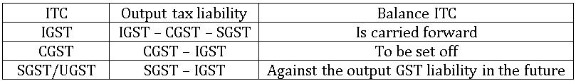
Utilization of ITC:

The Amount of ITC available to any registered dealer shall be utilized to reduce the out put tax liability in the sequence shown in the table.

E – ledgers under GST:
An E – ledger is an electronic form of a pass book available to all GST registrants on the GST portal. These are of three types:

(i) Electric cash ledger (ii) Electric credit ledger and (iii) Electric Liability Register

(i) Electric cash ledger: It contains the amounts of GST deposited in each to the government.

(ii) Electric credit ledger: It contains the balance of ITC available to the dealer.

(iii) Electric credit ledger: It contains all the Tax liability of the dealer.

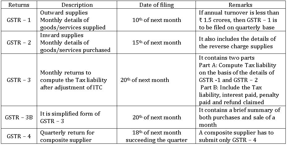
GST Returns:

These are the information provided from time to time by the dealer to the Government regarding the ITC, output Tax liability and the amounts of GST deposited.

A GST registered person has to submit the following returns:

E – Way bill:
E – Way bill is an electronic way bill that can be generated on the E – Way bill portal. A registered person can not transport goods whose value exceeds ₹ 50,000 in a vehicle without an e – way bill. When an E – way bill is generated, a unique e – way bill number (EBN) is allocated and is available to the supplier, the transporter and recipient. A dealer must generate an E – way bill if he has to transport them for returning to the supplier. 

2.Banking

 To encourage the habit of saving income groups, banks and post offices provide recurring deposit schemes.

Maturity period: An investor deposits a fixed amount every month for a fixed time period is called the maturity period,

Maturity value:  At the end of the maturity period, the investor gets the amount deposited with the interest. The total amount received by the investor is called Maturity value.

Interest =   

Where p is the principle

n is no. of months

r is the rate of interest

Maturity value = (p × n) + I

3.Shares and Dividend

Capital: The total amount of money needed to run the company is called Capital.

Nominal value (N.V): – The original value of a share is called the nominal value. It is also called as face value (F.V), printed value (P.V) or registered Value (R.V).

Market value: – The price of a share at a particular time is called market value (M.V). This value changes from time to time.

Shares: The whole capital is divided in to small units is called shares.

Share at par: – If the market value of a share is equal to face value of a share, then that share is called a share at par.

Share at a premium or Above par: – If the market value of a share is greater than the face value of the share then, the share is called share at a premium or above par.

Share at discount: – If the market value of a share is lesser than the face value of the share then, the share is called share at discount.

Dividend: – The profit distributed to the shareholders from a company at the end of the year is called a dividend.

The dividend is always calculated as the percentage of face value of the share.

Some formulae:

Note:

• The face value of a share always remains the same
• The market value of a share changes from time to time.
• Dividend is always paid on the face value of a share

 4. Linear In equations

Linear inequations: A statement of inequality between two expressions involving a single variable x with highest power one is called linear inequation.

Ex: 3x – 3 < 3x + 5; 2x + 10 ≥ x – 2 etc.

General forms of Inequations: The general forms of the linear inequations are: (i) ax + b < c   (ii) ax + by ≤ c    (iii)  ax + by ≥ c    (iv) ax + by > c, where a, b and c are real numbers and a ≠ 0.

Domain of the variable or Replacement Set: The set form which the value of the variable x is replaced in an inequation is called the Domain of the variable.

Solution set: The set of all whole values of x from the replacement set which satisfy the given inequation is called the solution set.

Ex: Solution set of x < 6, x ∈ N is {1, 2, 3, 4, 5}

Solution set of x ≤ 6, x ∈ W is {0, 1, 2, 3, 4, 5, 6}

Inequations – Properties:

• Adding the same number or expression to each side of an inequation does not change the inequality.

Ex: 3 < 5

Add 2 on both sides

3 + 2< 5 + 2

5 < 7 (no change in inequality)

• Subtracting the same number or expression to each side of an inequation does not change the inequality.

Ex: 3 < 5

subtract 2 on both sides

3 – 2 < 5 – 2

1 < 3 (no change in inequality)

• Multiplying or Dividing the same positive number or expression to each side of an inequation does not change the inequality.

Ex: 3 < 5

Multiply 2 on both sides

3 × 2< 5 × 2

6 < 10 (no change in inequality)

6 < 8

Divide 2 on both sides

6 ÷ 2< 8 ÷ 2

3< 4 (no change in inequality)

•Multiplying or Dividing the same negative number or expression to each side of an inequation can change(reverse) the inequality.

Ex: 3 < 5

Multiply 2 on both sides

3 × –2< 5 × –2

–6 > –10 (change in inequality)

6 < 8

Divide 2 on both sides

6 ÷ –2< 8 ÷ –2

–3 > –4 (change in inequality)

Note:

• a < b iff b > a
• a > b iff b < a

Ex: x < 4 ⇔ 4 > x

x > 3 ⇔ 3 < x

Method of solving Liner Inequations:

• Simplify both sides by removing group symbols and collecting like terms.
• Remove fractions by multiplying both sides by an appropriate factor.
• Collect all variable terms on one side and all constants on the other side of the inequality sign.
• Make the coefficient of the variable 1.
• Choose the solution set from the replacement set.

Ex: Solve the inequation 3x – 2 < 2 + x, x ∈ W

Sol: given in equation is

3x – 2 < 2 + x

Add 2 on both sides

3x – 2 + 2< 2 + x + 2

3x < 4 + x

3x – x < 4

2x < 4

Dividing both sides by 2

x < 2

∴ Solution set = { 0, 1}

5.Quadratic Equations

Quadratic Equation: An equation of the form ax² + bx + c = 0, where a, b, and c are real and a ≠ 0 is called a Quadratic equation in a variable ‘x’.

Ex: x ² – 3x + 4 = 0 is a quadratic equation in a variable ‘x’

t² + 5t = 6 is a quadratic equation in a variable ’t’

Roots of a quadratic equation: A number α is called a root of the quadratic equation ax² + bx + c = 0, if aα² + bα + c = 0.

Solution set:  The set of elements representing the roots of a quadratic equation is called solution set of the give quadratic equation.

Solving Quadratic equation by using Factorization met

hod:

Step – 1: Make the given equation into the standard form of ax² + bx + c = 0.

Step – 2: Factorise ax² + bx + c into two linear factors.

Step – 3: Put each linear factor equal to zero.

Step – 4: Solve these linear equations and get two roots of the given quadratic equation.

Ex: Solve x² – 3x – 4 = 0

x² – 4x + x – 4 = 0

x (x – 4) + 1 (x – 4) = 0

(x – 4) (x + 1) = 0

x – 4 = 0 or x + 1 = 0

x = 4 or x =– 1

∴ Solution set = {– 1, 4}

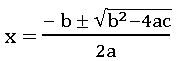
Solving Quadratic equation by using Formula:

The roots of the quadratic equation ax² + bx + c = 0 are:

Ex: Solve x² – 3x – 4 = 0

Sol: Given equation is x² – 3x – 4 = 0

Compare with ax² + bx + c = 0

a = 1, b = – 3, c = – 4

x = 4 or x = – 1

∴ Solution set = {– 1, 4}

Nature of the roots:

Discriminant: – For a quadratic equation ax² + bx + c = 0, b² – 4ac is called discriminant.

(i) If b² – 4ac > 0, then roots are real and un equal.

     Case – 1: b² – 4ac > 0 and it is a perfect square, then roots are rational and unequal.  

    Case – 2: b² – 4ac > 0 and it is not a perfect square, then roots are irrational and unequal.     

(ii) If b² – 4ac = 0, then roots are equal and real.

(iii) b² – 4ac < 0, then roots are imaginary and un equal.

6.Problems on Quadratic equations

To solve word problems and determine unknown values, by forming quadratic equations from the information given and solving them by using methods of solving Quadratic equation.

The problems may be based on numbers, ages, time and work, time and distances, mensuration etc.

Method of Solving word problems in Quadratic equation:

Step – 1: Read the given problem carefully and assume the unknown be x.

Step – 2: Translate the given statement and form a quadratic equation in x.

Step – 3: Solve for x.

7.Ratio and Proportion

Ratio: Comparing two quantities of same kind by using division is called a ratio.

The ratio between two quantities ‘a’ and ‘b’ is written as a : b and read as ‘a is to b’

In the ratio a : b, ‘a’  is called ‘first term’ or ‘antecedent’ and ‘b’ is called ‘second term’ or ‘consequent’.

Note:  The value of a ratio remains un changed if both of its terms are multiplied or divided by the same number, which is not a zero.

Lowest terms of a Ratio:

In the ratio a : b, if a, b have no common factor except 1, then we say that a : b is in lowest terms.

Ex: 4 : 12 = 1 : 3 ( lowest terms)

Comparison of Ratios:  

• (a : b) > (c : d) ⇔ ad > bc
• (a : b) = (c : d) ⇔ ad = bc
• (a : b) < (c : d) ⇔ ad < bc

Proportion:

An equality of ratios is called a proportion.

a, b, c and d are said to be in proportion if a : b = c : d and we write as a : b : : c : d.

a and d are ‘extremes’, b and c are ‘means’

product of extremes = product of means

Continued proportion: If a, b, c, d, e and f are in continued proportion, then

Mean proportion:  If then b² = ac or b =  , b is called mean proportion between a and b.

Third proportional: If a : b = b : c, then c is called third proportional to a and b.

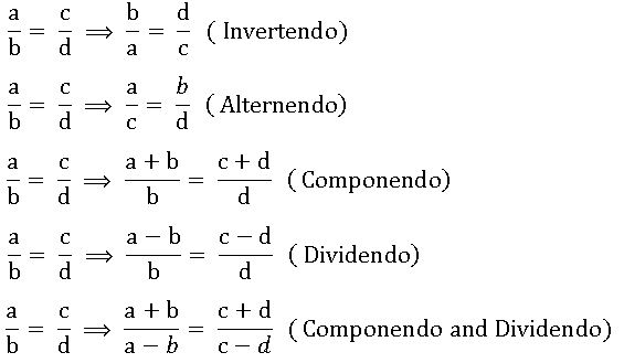
Note: 

Results on Ratio and Proportion:

8.Remainder Theorem and Factor Theorem

Polynomial: An expression of the form p(x) = a₀ xⁿ + a₁ x^n-1 + a₂ x^n-2 + …+ a_n-1 x + a_n, where a₀, a₁, …, a_n are real numbers and a₀ ≠ 0. Is called a polynomial of degree n.

Value of a polynomial: The value of a polynomial p(x) at x = a is obtained by substituting x = a in the given polynomial and is denoted by p(a).

Ex: If p(x) = 2x + 3, then find the value of p (1), p (0).

Sol: given p(x) = 2x + 3

p (1) = 2 (1) + 3 = 2 + 3 = 5

p (0) = 2 (0) + 3 = 0 + 3 = 3

Division algorithm: On dividing a polynomial p(x) by a polynomial g(x), there exist quotient polynomial q(x) and remainder polynomial r(x) then

p(x) = g(x) q(x) + r(x)

p(x) is dividend; g(x) is divisor; q(x) is quotient; r(x) is remainder.

Remainder theorem:

If a polynomial p(x) is divided by (x – a), then the remainder is p(a).

Ex: If p(x) = 2x – 1 is divided by (x – 3), then find reminder.

Sol: Given p(x) = 2x – 1

Remainder = p (3)

= 2(3) – 1

= 6 – 1 = 5

∴ remainder is 5

Note:

• If p(x) is divided by (x + a), then the remainder is p (– a).
• If p(x) is divided by (ax + b), then remainder is .
• If p(x) is divided by (ax – b), then remainder is .

Factor theorem: Let p(x) be a polynomial and ‘a’ be given real number, then (x – a) is a factor of p(x) ⇔ p(a) = 0.

Note:

• If (x + a) is the factor of p(x), then p (– a) = 0.
• If (ax + b) is the factor of p(x), then  = 0.
•  If (ax – b) is the factor of p(x),    = 0

9. Matrices

Matrix: A rectangular arrangement of numbers in the form of horizontal and vertical lines and enclosed by the brackets [ ] or parenthesis ( ), is called a matrix.

The horizontal lines in a matrix are called its rows.

The vertical lines in a matrix are called its columns.

Oder of Matrix: A matrix having ‘m’ rows and ‘n’ columns is said to be of order m x n read as m by n.

Ex: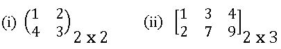   

Elements of a matrix:

An element of a matrix appearing in the i^th row and j^th column is called the (i, j)^th element of the matrix and it is denoted by a_ij.

A = [a_ij]_{m × n}

A =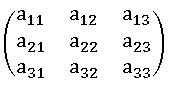

a₁₁ means element in first row and first column

a₁₂ means element in first row and second column

a₂₂ means element in second row and second column

a₃₂ means element in third row and second column

and so on.

Types of Matrices

Row matrix & column Matrix: A matrix with only one row s called a row matrix and a matrix with only one column is called column matrix.

Ex: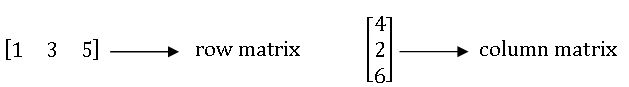

Rectangular Matrix: A matrix in which the no. of rows is not equal to no. of columns is called Rectangular matrix.

Ex:

Square Matrix: A matrix in which the no. of rows is equal to no. of columns is called square matrix.

Ex:

 Diagonal Matrix: If each non-diagonal elements of a square matrix is ‘zero’ then the matrix is called diagonal matrix.

Ex: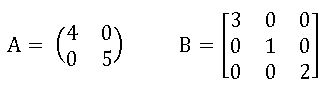

Identity Matrix or Unit Matrix: If each of non-diagonal elements of a square matrix is ‘zero’ and all diagonal elements are equal to ‘1’, then that matrix is called unit matrix

Ex: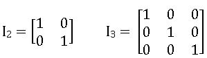

Null Matrix or Zero Matrix: If each element of a matrix is zero, then it is called null matrix.

Ex: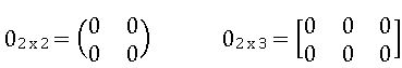  

Equality of matrices: matrices A and B are said to be equal if A and B of the same order and the corresponding elements of A and B are equal.

Ex: If 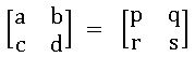 ⟹ a=p; b = q; c = r; d = s

Comparing Matrices: Comparison of two matrices is possible, if they have same order.

Transpose of Matrix: If A = [a_ij] is an m x n matrix, then the matrix obtained by interchanging the rows and columns is called the transpose of A. It is denoted by   A^T.

Ex: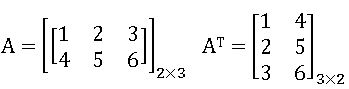

Addition of Matrices: If A and B are two matrices of the same order, then their sum A + B is the matrix obtained by adding the corresponding elements of A and B.

Ex:

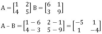
Subtraction of Matrices: If A and B are two matrices of the same order, then their difference A + B is the matrix obtained by subtracting the elements of B from the corresponding elements of A.

Ex:   

Product of Matrices:

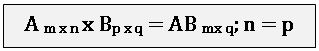
Let A = [a_ik]_mxn and B = [b_kj]_nxp be two matrices, then the matrix C = [c_ij]_mxp   where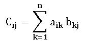

Note: Matrix multiplication of two matrices is possible when no. of columns of first matrix is equal to no. of rows of second matrix.

10. Arithmetic Progressions

Sequence:  The numbers which are arranged in a different order to some definite rule are said to form a sequence.

Ex: 1, 2, 3, ……

2, 4, 6, 8, ….

2, 4, 8, 16, …

Arithmetic Progression (A.P.):

A sequence in which each term differ from its preceding term by a constant is called an Arithmetic Progression (A.P.). The constant difference is called the common difference.

Terms: a, a + d, a + 2d…, a + (n – 1) d

First term: a

Common Difference: d = a₂ – a₁ = a₃ – a₂ = … = a_n – a_{n -1}

n^th term: T_n = a + (n – 1) d

Sum of the n terms of A.P.:         

 Sum of the n terms of A.P. is

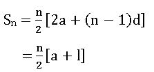
Where a is first term and l is last term.

To find the n^th term from the end of an A.P.:

Let a be first term, d be the common difference and ‘l’ be the last term of a given A.P. then its n^th term from the end is l – (n – 1) d .

11. Geometric Progressions

Terms: a, a r, a r²…, a r^{n – 1}  

First term: a

Common ratio:   

n^th term: T_n = a r^{n – 1}  

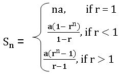
Sum of the n terms of G.P.:

Sum of the n terms of G.P. is

To find the n^th term from the end of an G.P.:

Let a be first term, r be the common ratio and ‘l’ be the last term of a given G.P. then its n^th term from the end is

12. Reflection

Coordinate Axes:

The position of the point in a plane is determined by two fixed mutually perpendicular lines XOX’ and YOY’ intersecting each other at ‘O’. These lines are called coordinate axes.

The horizontal line XOX’ is called X – axis.

The vertical line YOY’ is called Y – axis.

The point of intersection axes is called ‘origin’.

Coordinates of a point:

Let P be any point on the plane, the distance of P from X – axis is ‘x’ units and the distance of P from Y – axis is ‘y’ units, then we say that coordinates of P are (x, y).

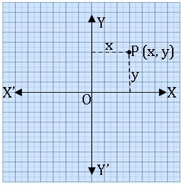
x is called x coordinate or abscissa of P

y is called y coordinate or ordinate of P

The distance of any point on X – axis from X – axis is 0

∴ Any point on the X – axis is (x, 0)

The distance of any point on Y – axis from Y – axis is 0

∴ Any point on the Y – axis is (0, y).

The coordinates of the origin O are (0, 0).

The equation of X – axis is y = 0.

The equation of any line parallel to X – axis is y = k, where k is the distance from X – axis.

The equation of Y – axis is x = 0.

The equation of any line parallel to Y – axis is x = k, where k is the distance from Y – axis.

Reflection

Image of an object in a mirror: When an object is placed in front of a plane mirror, then its image is formed at the same distance behind the mirror as the distance of the object from the mirror.

Image of a point in a line:

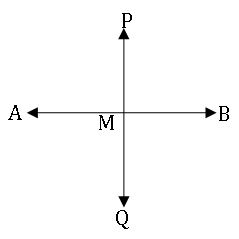
Let P be a point and AB is a given line. Draw PM perpendicular to AB and produce PM

to Q such that PM = QM, then Q is called image of P with respect to the line AB.

Reflection of a point in a line:

Assume the given line as a mirror, the image of a given point is called the reflection of that point in the given line.

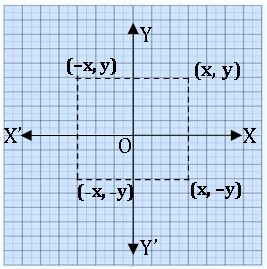
Reflection of P (x, y) in X – axis is P (x, –y) ⇒ R_x (x, y) = (x, –y)

Reflection of P (x, y) in Y – axis is P (–x, y) ⇒ R_x (x, y) = (–x, y)

Reflection of P (x, y) in the origin is P (–x, –y) ⇒ R_x (x, y) = (–x, –y)

Combination of Reflection:

• R_x. R_y = R_y. R_x = R_o
• R_x. R_o = R_o. R_x = R_y
• R_y. R_o = R_o. R_y = R_x

Invariant Points: A point P is said to be invariant in a given line if the image of P (x, y) in that line is P (x, y).

13. Section and Mid – Point Formula

Section formula: If P (x, y) divides the line segment joining the points A (x₁, y₁) and B (x₂, y₂) in the ratio m : n, then

P (x, y) =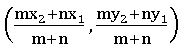

Mid pint Formula:

The mid-point of the line segment joining the points A (x₁, y₁) and B (x₂, y₂) is

Centroid of the triangle:

The point of concurrence of medians of a triangle is called centroid of the triangle. It is denoted by G.

The centroid of the triangle formed by the vertices A (x₁, x₂), B (x₂, y₂) and C (x₃, y₃) is

G =

14. Equation of a Straight line

Inclination of a line: The angle of inclination of a line is the angle θ which is the part of the line above the X – axis makes with the positive direction of X – axis and measured in anticlockwise direction.

Horizontal line: A line which is parallel to X – axis is called horizontal line.

Vertical line: A line which is parallel to Y – axis is called vertical line.

Oblique line: A line which is neither parallel to X – axis nor parallel to Y – axis is called an oblique line.

Slope or Gradiant of a line:

A line makes an angle θ with the positive direction of x – axis then tan θ is called the slope of the line, it is denoted by ‘m’

m = tan θ

1. Slope of the x- axis is zero.
2. Slope of any line parallel to x- axis is zero.
3. Slope of y- axis is undefined.
4. Slope of any line parallel to y- axis is also undefined.
5. Slope of the line joining the points A (x₁, y₁) and B (x₂, y₂) is

6. Slope of the line ax + by + c = 0 is  =

Condition for collinearity: If three points A, B and C are lies on the same line then they are collinear points.

Condition for the collinearity is slope of AB = Slope of BC = slope of AC

Types of equation of a straight line:

• Equation of x- axis is y = 0.
• Equation of any line parallel to x – axis is y = k, where k is distance from above or below the x- axis.
• Equation of y- axis is x = 0.
• Equation of any line parallel to y – axis is x = k, where k is distance from left or right side of the y- axis.

Slope intercept form:

The equation of the line with slope m and y- intercept ‘c’ is y = mx + c.

Slope point form:

The equation of the line passing through the point (x₁, y₁) with slope ‘m’ is

y – y₁ = m (x – x₁)

Two points form:

The equation of the line passing through the points (x₁, y₁) and (x₂, y₂) is

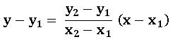
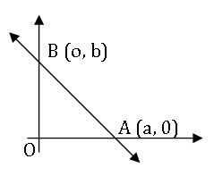
Intercept form:

The equation of the line with x- intercept a, y – intercept b is

Note: –

1. If two lines are parallel then their slopes are equal

                            m₁ = m₂

2. If two lines are perpendicular then product of their slopes is – 1

         m₁ × m₂ = – 1

          slope of a line perpendicular to a line AB =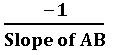

 15. Similarity

Similar figures: If two figures have same shape but not in size, then they are similar.

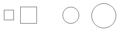
Similarity as a Size transformation:

It is the process in which a given figure is enlarged or reduced by a scale factor ‘k’, such that the resulting figure is similar to the given figure.

The given figure is called an ‘object’ and the resulting figure is called its ‘image’

Properties of size transformation:

Let ‘k’ be the scale factor of a given size transformation, then

If k > 1, then the transformation is enlargement.

If k = 1, then the transformation is identity transformation.

If k < 1, then the transformation is reduced.

Note:

• Each side if the resulting figure = k times the corresponding side of the given figure.
• Area of the resulting figure = k² × (Area of the given figure).
• Volume of the resulting figure = k³ × (Volume of given figure).

Model: The model of a plane figure and the actual figure are similar to one another.

Let the model of the plane figure drawn to the scale 1 : n, then scale factor k =  .

• Length of the model = k × (length of the actual figure)
• Area of the model = k² × (Area of the actual figure).
• Volume of the model = k³ × (Volume of actual figure).

Map: The model of a plane figure and the actual figure are similar to one another.

Let the Map of the plane drawn to the scale 1 : n, then scale factor k =  .

• Length of the map = k × (Actual length)
• Area of the model = k² × (Actual area).

16. Similarity of Triangles

Similar triangles: Two triangles are said to be similar If: (i) their corresponding angles are equal and (ii) their corresponding sides are in proportional (in same ratio).

If ∆ABC ~ ∆DEF, then

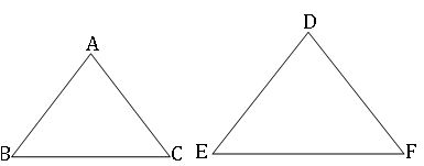
• ∠A = ∠D, ∠B = ∠E and ∠C = ∠F
• 

 Here k is scale factor, (i) if k > 1, then we get enlarged figures (ii) if k = 1, then we get congruent figures (iii) if k < 1, then we get reduced figures.

Axioms of Similar Triangles

SAS – Axiom:

If two triangles have a pair of corresponding angles equal and the corresponding sides including them proportional, then the triangle is similar.

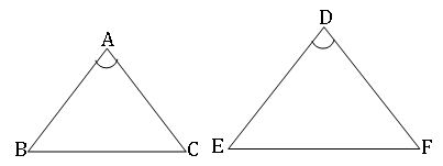
In ∆ABC and ∆DEF, ∠A = ∠D and

AA – Axiom : If two triangles have two pairs of corresponding angles equal, then the triangles are equal.

SSS – Axiom: If two triangles have their three sides of corresponding sides proportional, then the triangles are similar.

Basic proportionality Theorem:

In a triangle a line drawn parallel to one side divides the other two sides in the same ratio (proportional).

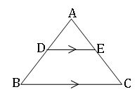
In ∆ ABC, DE ∥ BC ⇒

Converse of Basic proportionality Theorem:

If a line divides any two sides of a triangle proportionally, the line is parallel to the third side.

In ∆ ABC,  ⇒ DE ∥ BC.

∎ Ina triangle the internal bisector of an angle divides the opposite side in the ratio of the sides containing the angle.

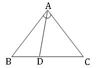
In ∆ ABC, AD bisects ∠A then

∎ The areas of two similar triangles are proportional to the squares of their corresponding sides.

If ∆ABC ~ ∆DEF, then

∎ The areas of two similar triangles are proportional to the squares of their corresponding medians.

If ∆ABC ~ ∆DEF and AM, DN are medians of   ∆ABC and ∆DEF respectively then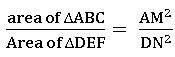

∎ The areas of two similar triangles are proportional to the squares of their corresponding altitudes.

If ∆ABC ~ ∆DEF and AM, DN are altitudes of ∆ABC and ∆DEF respectively then

17. Loci

Locus: Locus is the path traced out by a moving point which moves according to some given geometrical conditions.

The plural form of Locus is ‘Loci’ read as ‘losai’

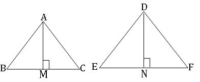
∎ The locus of the point which is equidistance from two given fixed points is the perpendicular bisector of the line segment joining the given fixed       points.

∎ Every point on the perpendicular bisector of AB is equidistance from A and B.

∎ The locus of the point which is equidistance from two intersecting lines is the pair of lines bisecting the angles formed by the given lines.

∎Every point on the angular bisector of two intersecting lines is equidistance from the lines.

18. Angle and Cyclic Properties of a Circle

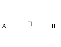
∎ The angle subtended by an arc of a circle is double the angle subtended by it at any point on the circle.

∠AOB = 2 ∠ACB

∎ Angles in a same segment of a circle are equal.

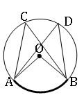
∠ACB = ∠ADB

∎ The angle in a semi-circle is 90⁰

∎ If an arc of a circle subtends a right angle at any point on the remaining part of the circle, then the arc is semi-circle.

Cyclic Quadrilateral:

A quadrilateral is said to be cyclic if all the vertices passing through the circle.

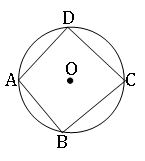
The opposite angles of cyclic quadrilateral are supplementary.

∎ If pair of opposite angles of a quadrilateral are supplementary, then the quadrilateral is cyclic.

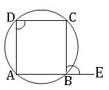
∎ The exterior angle of a cyclic quadrilateral is equal to the interior opposite angle.

 ∎ Every cyclic parallelogram is a rectangle.

∎ An isosceles trapezium is always cyclic and its diagonals are equal.

∎ The mid-point of hypotenuse of a right-angled triangle is equidistance from its vertices.

19. Tangent Properties of Circles

Tangent: A line which intersect the circle at only one point is called Tangent to the circle.

∎ The tangent at any point of a circle and radius through the point are perpendicular to each other.

∎ If two tangents are drawn to a circle from an exterior point, then

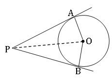
• The tangents are equal in length.
• The tangents subtend equal angle at the centre.
• The tangents are equally inclined to the line joining the point and the centre if the circle.

Intersecting Chord and Tangents

Segment of a chord:

If P is a point on a chord AB of a circle, then we say that P divides AB internally into two segments PA and PB.

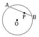
If AB is a chord of a circle and P is a point on AB produced, we say that P divides AB externally into two segments PA and PB.

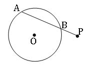
∎ If two chords of a circle intersect internally or externally, then the product of the lengths of their segments are equal.

Alternate segments:

In the given figure APB is a tangent to the circle at point at a point P and PQ is a chord

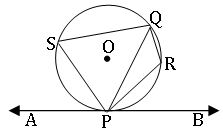
The chord PQ divides the circle into two segments PSR and PSQ are called alternate segments.

The angle between a tangent and a chord through the point of contact is equal to an angle in the alternate segment.

∠QPB = ∠PSQ and ∠APQ = ∠PRQ

20. Constructions

21. Volume and Surface Area of Solids

Cylinder:

Solids like circular pillars, circular pipes, circular pencils etc. are said to be in cylindrical shape.

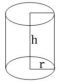
Radius of the base = r

Height of the cylinder = h

Curved surface area = 2πrh sq. units

Total surface area = 2πr (r + h) sq. units

Volume = πr²h cubic. units

Hollow Cylinder:

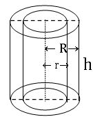
External radius = R

Internal radius = r

Height = h

Thickness of the cylinder = R – r

Area of cross section = π (R² – r²) sq. units

Volume of material = πh (R² – r²) cubic. units

Curved surface area = 2πh (R+ r) sq. units

Total surface area = 2π (Rh + rh + R² – r²) sq. units

Cone:

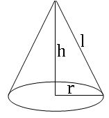
Radius of the base = r

Height of the cylinder = h

Slant height = l

l² = r² + h² ⇒ l =

Curved surface area = πrl sq. units

Total surface area = πr (r + l) sq. units

Volume = πr²h cubic. Units

Sphere:

Objectives like football, throwball, etc. are said to be the shape of sphere.

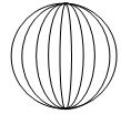
Radius of Sphere = r

Surface area = 4πr² sq. units

Volume = πr³ cubic. Units

Spherical Shell:  

The solid enclosed between two concentric spheres is called spherical shell

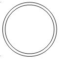
External radius = R

Internal radius = r

Thickness of the cylinder = R – r

Volume of the material =  π (R³ – r³) cubic. Units

Hemi sphere:

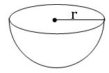
Radius of hemisphere = r

Curved Surface area = 2πr² sq. units

Surface area = 3πr² sq. units

Volume = πr³ cubic. Units

22.Trigonometrical Identities

The word Trigonometry derived from Greek word, tri → three, gonia → angle and metron → to measure.

Angle: – The figure formed by two rays meeting at a common end point is an angle.

Naming the sides in a right-angled triangle:

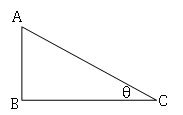
AB = Perpendicular =opposite side of θ (opp)

BC = Base = adjacent side of θ(adj)

AC is hypotenuse (hyp)

Trigonometric ratios:

Quotient relations:

Trigonometric Identities:
(i) sin²θ + cos²θ = 1          (ii) sec²θ − tan²θ = 1        (iii) cosec²θ − cot²θ = 1

∎ sin²θ = 1 − cos²θ; cos²θ = 1 – sin²θ

∎ sec²θ = tan²θ + 1; sec²θ – 1 =tan²θ

∎ Cosec²θ = Cot²θ + 1; Cosec²θ – 1 = Cot²θ

Trigonometric tables:

A trigonometric Table Consist of three parts:

• A column on the extreme left containing degree from 0⁰ to 89⁰.
• The columns headed by 0’, 6’, 12’, 18’, 24’, 30’, 36’, 42’, 48’ and 54’.
• Five columns of mean differences, headed by 1’, 2’, 3’, 4’ and 5’

Note:

• The mean difference is added in case of ‘sines’, ‘tangents’ and ‘secants’
• The mean difference is subtracted in case of ‘cosines’, ‘cotangents’ and ‘cosecants’

Relation between degrees and minutes:

1⁰ = 60’⇒ 1’ =

Trigonometric Tables Charts:

By clicking below you get Sin, Cosine and Tangent Tables

 Click here

Loading...

Taking too long?

Reload document

| Open in new tab

23. Heights and Distances

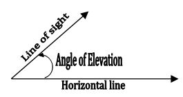
Horizontal line: A line which is parallel to earth from observation point to object is horizontal line
Line of sight: The line of sight is the line drawn from the eye of an observer to the point in the object viewed by the observer.

Angle of elevation: The line of sight is above the horizontal line and angle between the line of sight and horizontal line is called angle of elevation.

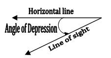
Angle of depression: The line of sight is below the horizontal line and angle between the line of sight and horizontal line is called angle of depression.

Solving procedure:

∎All the objects such as tower, trees, buildings, ships, mountains etc. shall be consider as linear for mathematical convenience.

∎The angle of elevation or angle of depression is considered with reference to the horizontal line.

∎The height of observer neglected, if it is not given in the problem.

∎To find heights and distances we need to draw figures and with the help of these figures we can solve the problems.

24. Graphical Representation of Statistical Data

Data: A set of given facts in numerical figures is called data.

Frequency: The number of times an observation occurs is called its frequency.

Frequency Distribution: The tabular arrangement of data showing the frequency of each observation is called its frequency distribution.

Class interval: Each group into which the raw data is condensed is called a class interval.

Class limits: Each class interval is bounded by two figures is called Class limits.

Left side part of class limit is called ‘Lower limit’

Right side part of class limit is called ‘Upper limit’

Inclusive form:  In each class, the data related to both the lower and upper limits are included in the same class, is called Inclusive form.

Ex: 1 – 10, 11 – 20, 21 – 30 etc.

Exclusive form: In each class, the data related to the upper limits are excluded is called Exclusive form.

Ex: 0 – 10, 10 – 20, 20 – 30 etc.

Class size = upper limit – lower limit

Class mark =  [lower limit + upper limit]

Note:

In an inclusive form, Adjustment factor =  [lower limit of one class – upper limit of previous class]

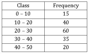
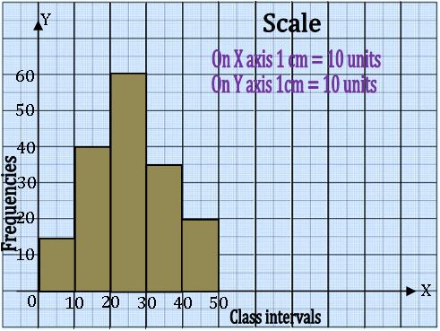
Histogram:  A histogram is a graphical representation of a frequency distribution in an exclusive form, in the form of rectangles with class interval as bases and the corresponding frequencies as heights

Method of drawing a Histogram:

Step-1:  If the given frequency distribution is in inclusive, then convert them into the exclusive form

Step-2: Choose a suitable scale on the X – axis and mark the class intervals on it.

Step-3: Choose a suitable scale on the Y – axis and mark the frequencies on it.

Step-4: Draw rectangle with class intervals as bases and the corresponding frequencies as the corresponding heights.

Example:

Frequency polygon:

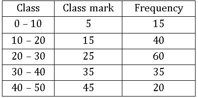
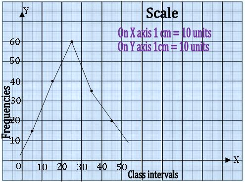
 Let x₁, x₂, x₃, …, x_n be the class marks of the given frequency distribution and f₁, f₂, f₃, …, f_n be the corresponding frequencies, then plot the points (x₁, f₁), (x₂, f₂), …. (x_n, f_n) on a graph paper and join these points by a line segment. complete the diagram in the form of polygon by taking two or more classes.

Example:

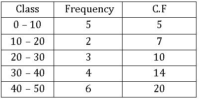
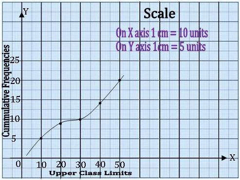
Cumulative Frequency curve or Ogive:

In order to represent a frequency distribution by an Ogive, we mark the upper class along X– axis and the corresponding cumulative frequencies along Y – axis and join these points by free hand curve, called Ogive.

Example:

25. Measures of Central Tendency

Average of a Data:

For a given data a single value of the variable representing the entire data which describes the characteristics of the data is called average of the data.

An average tends to lie centrally with the values of the variable arranged in ascending order of magnitude. So, we call an average a measure of central tendency of the data.

Three measures of central tendency are:   (i) Mean   (ii) Median  and (iii) Mode

Average of a Data:

For a given data a single value of the variable representing the entire data which describes the characteristics of the data is called average of the data.

An average tends to lie centrally with the values of the variable arranged in ascending order of magnitude. So, we call an average a measure of central tendency of the data.

Three measures of central tendency are:   (i) Mean   (ii) Median  and (iii) Mode

Mean

Mean for Un Grouped data:

The mean of ‘n’ observations x₁, x₂, x₃, …, x_n is

Mean =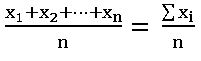

The Symbol Σ is called ‘sigma’ stands for summation of the data.

Note:

If the mean of a data x₁, x_{2, …} x_n is m, then

• Mean of (x₁+k), (x₂ + k), …. (x_n + k) = m + k
• Mean of (x₁−k), (x₂ − k), …. (x_n − k) = m −k
• Mean of (k x₁), (k x₂), …. (k x_n) = k m

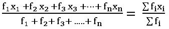
If x₁, x₂, …. x_n are of n observations occurs f₁, f₂, …. f_n times respectively then mean is

Mean of grouped data:

Methods of finding mean:

Class mark (mid value) =

 Direct method: ;  x_i is class mark of i^th class, f_i is frequency of class.

Assumed mean method: 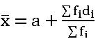;  d_i = x_i – a and a is assumed mean.

Step – deviation method: 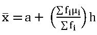 ; 𝛍_i =  , h is class size.

26. Median, Quartile and Mode

Median

Median is the middle most observation of given data.

For un grouped data:

First, we arrange given observations into ascending or descending order.

If n is odd median =  observation.

If n is even median =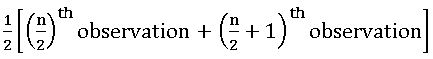

For grouped data:

Median =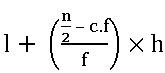 , where

l is the lower boundary of median class

f is the frequency of median class

c.f is the preceding cumulative frequency of the median class

h is the class size

Quartiles

The observations which divides the whole set of observations into 4 equal parts are known as Quartiles.

Lower Quartile (First Quartile): If the variates are arranged in ascending order, then the observations lying midway between the lower extreme and the median is called the Lower Quartile. It is denoted by Q₁.

If n is Even Q₁ =   observation

If n is Odd Q₁ =  observation

Middle Quartile: The middle Quartile is the median, denoted by Q₂.

Upper Quartile (Third Quartile): If the variates are arranged in ascending order, then the observations lying midway between and the median the upper extreme is called the Upper Quartile. It is denoted by Q₃.

If n is Even Q =  observation

If n is Odd Q₁ = observation

Range: The difference between the biggest and the smallest observations is called the Range.

Interquartile Range: The difference between the upper quartile and Lower quartile is called the inter quartile.

Range = Q₃ – Q₂

Semi – interquartile range:

Semi – interquartile Range = ½ [ Q₃ – Q₂]

Estimating median:

Step 1: If the given frequency distribution is not continuous, convert into the continuous form.

Step 2: Prepare the cumulative frequency table.

Step 3: Draw Ogive for the cumulative frequency distribution given above

Step 4: Let sum of the frequencies = N.

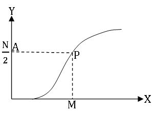
Step 5: Mark a point A on Y- axis corresponding to

Step 6: From A draw Horizontal line to meet Ogive curve at P. From P draw a vertical line PM to meet X – axis at M. Then the abscissa of M gives the Median.

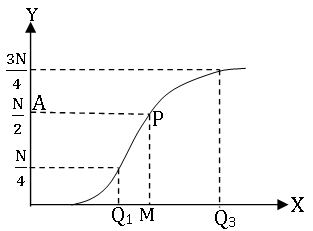
Estimating Q₁ and Q₂:

To locate the value of Q₁ on Ogive curve, we mark the point along

Y – axis, corresponding to  and proceed similarly.

To locate the value of Q₃ on Ogive curve, we mark the point along

Y – axis, corresponding to  and proceed similarly.

Mode

The value of a data which is occurred most frequently is called Mode.

Modal class: The class with maximum frequency is called the Modal class.

Estimation of Mode from Histogram:

Step 1: If the given frequency distribution is not continuous, convert it into a continuous form.

Step 2: Draw a histogram to represent the above data.

Step 3: from the upper corner of the highest rectangle, draw line segments

To meet the opposite corners of adjacent rectangles, diagonally

Let these line segments intersect at P.

Step 4: Draw PM perpendicular to X-axis at M, Then the abscissa of M is The Mode

27. Probability

J Cordon Italian mathematician wrote the first book on probability named “the book of games and chance”.

Probability:

It is the concept which numerically measures the degree of certainty of the occurrence of an event.

Some words in probability:

Experiment: A repeatable procedure with a set of possible results.

Trial: By a trial, we mean experimenting.

Outcome: a possible result of an experiment.

Sample space: All the possible outcomes of an experiment.

Sample point: Just one of the possible outcomes.

Event: One or more outcomes of an experiment.

Probability of occurrence of an Event (Classical definition):

In a random experiment Let S be the sample space and E be the event, then E ⊆ S. The probability of occurrence of E is defined as:

P(E) = 

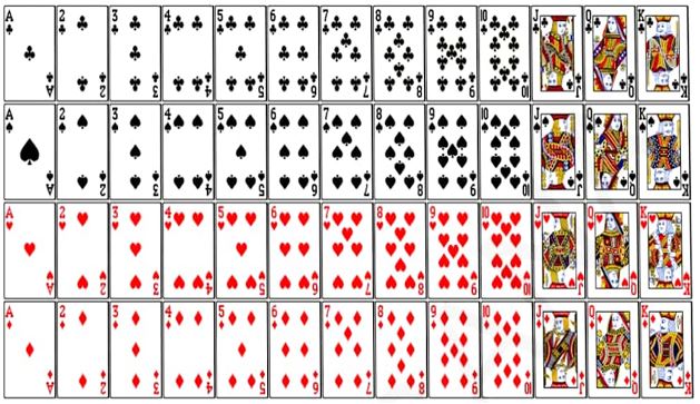
Deck of cards: A deck of playing cards consists of 52 cards which are divided into 4 suits of 13 cards each. They are black spade     , black clubs, red heart     and red diamond       . The cards in each suit are: 2, 3, 4, 5, 6, 7, 8, 9 ,10, Ace, Jack, Queen and King. Jack, Queen and King are called face (picture) cards.

Impossible event: If there is no probability of an event to occur then it is impossible event. Its probability is zero.

Sure or certain event: If the probability of an event is 1 then it is sure or certain event.

Complimentary event: Let E denote the event, ‘not E’ is called complimentary event of E. It is denoted by  . P ( ) = 1 – P(E) ⟹ P ( ) +P(E) = 1.

 0 ≤ P(E) ≤ 1

Visit my Youtube Channel: Click on Below Logo