TS Inter Second Year Maths 2A concept
TS Inter Second Year Maths : This note is designed by ‘Basics in Maths’ team. These notes to do help the TS intermediate second year Maths students fall in love with mathematics and overcome the fear.
These notes cover all the topics covered in the TS I.P.E second year maths 2A syllabus and include plenty of formulae and concept to help you solve all the types of Inter Math problems asked in the I.P.E and entrance examinations.
1. COMPLEX NUMBERS
• The equation x2 + 1 = 0 has no roots in real number system.
∴ scientists imagined a number ‘i’ such that i2 = − 1.
Complex number: if x, y are any two real numbers then the general form of the complex number is
z = x + i y; where x real part and y is imaginary part.
∗ z = x + iy can be written as (x, y)
∗If z1 = x1 + i y1, z2 = x2 + i y2, then
∗ z1 + z2 = (x1 + x2, y1 + y2) = (x1 + x2) + i (y1 + y2)
∗ z1 − z2 = (x1 − x2, y1 − y2) = (x1 − x2) + i (y1 − y2)
∗ z1∙ z2 = (x1 x2 −y1 y2, x1y2 + x2y1) = (x1x2 −y1 y2) + i (x1y2 +x2 y1)
∗ z1/ z2 = (x1x2 + y1 y2/x22 +y22, x2 y1 – x1y2/ x22 +y22)
= (x1x2 + y1 y2/x22 +y22) + i (x2 y1 – x1y2/ x22 +y22)
Multiplicative inverse of complex number:
Multiplicative inverse of complex number z is 1/z.
z = x + i y then 1/z = x – i y/ x2 + y2
Conjugate complex number:
- The complex numbers x + iy, x – iy are called conjugate complex numbers.
- The sum and product of two conjugate complex numbers are real.
- If z1, z2 are two complex numbers then

Modulus and amplitude of complex number:
Modulus: – If z = x + iy, then the non-negative real number![]() is called the modulus of z and it is denoted by or ‘r’.
is called the modulus of z and it is denoted by or ‘r’.
Amplitude: – The complex number z = x + i y is represented by the point P (x, y) on the XOY plane. ∠XOP = θ is called amplitude of z or argument of z.
∗ x = r cosθ, y = r sinθ
⇒ x2 + y2 = r2 cos2θ + r2 sin2θ = r2 (cos2θ + sin2θ) = r2(1)
⇒ x2 + y2 = r2
⇒ r = ![]() and
and ![]() = r.
= r.
∗ Arg (z) = tan−1(y/x)
∗ Arg (z1.z2) = Arg (z1) + Arg (z2) + nπ for some n ∈ { −1, 0, 1}
∗ Arg(z1/z2) = Arg (z1) − Arg (z2) + nπ for some n ∈ { −1, 0, 1}
Argand plane: The plane containing all complex numbers is called the Argand plane. This was introduced by the mathematician Gauss (1777-1855), who first thought that complex numbers can be represented as a two-dimensional plane.

The square root of a complex number:

2.DE- MOIVER’S THEOREM
De- Moiver’s theorem: For any integer n and real number θ, (cosθ + i sinθ) n = cos nθ + i sin nθ.
→ cos α + i sin α can be written as cis α
→ cis α.cis β= cis (α + β)
→ 1/cisα = cis(-α)
→ cisα/cisβ = cis (α – β)
⟹ (cosθ + i sinθ) -n = cos nθ – i sin nθ
⟹ (cosθ + i sin θ) (cosθ – i sin θ) = cos2θ – i2 sin2θ = cos2θ + sin2θ = 1.
→ cosθ + i sin θ = 1/ cosθ – i sin θ and cosθ – i sin θ = 1/ cosθ + i sin θ
⟹ (cosθ – i sin θ) n = (1/ (cosθ –+i sin θ)) n = (cosθ + i sin θ)-n = cos nθ – i sin nθ
nth root of a complex number: let n be a positive integer and z0 ≠ 0 be a given complex number. Any complex number z satisfying z n = z0 is called an nth root of z0. It is denoted by z01/n or![]()
⟹ let z = r (cosθ + i sin θ) ≠ 0 and n be a positive integer. For k∈ {0, 1, 2, 3…, (n – 1)} let ![]() . Then a0, a1, a2, …, an-1 are all n distinct nth roots of z and any nth root of z is coincide with one of them.
. Then a0, a1, a2, …, an-1 are all n distinct nth roots of z and any nth root of z is coincide with one of them.
nth root of unity: Let n be a positive integer greater than 1 and
![]()
Note:
- The sum of the nth roots of unity is zero.
- The product of nth roots of unity is (– 1) n – 1.
- The nth roots of unity 1, ω, ω2, …, ωn-1 are in geometric progression with common ratio ω.
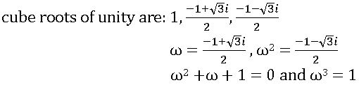
Cube root of unity:
x3 – 1 = 0 ⇒ x3 = 1
x =11/3
3.QUADRATIC EXPRESSIONS
Quadratic Expression: If a, b, c are real or complex numbers and a ≠ 0, then the expression ax2 + bx + c is called a quadratic expression in variable ‘x’.
∎ A complex number α is said to be a zero of the quadratic expression ax2 + bx + c if aα2 + bα + c = 0.
Quadratic Equation: If a, b, c are real or complex numbers and a ≠ 0, then ax2 + bx + c = 0 is called a quadratic equation in variable ‘x’.
∎ A complex number α is said to be root or solution of the quadratic equation ax2 + bx + c = o if aα2 + bα + c = 0.
The roots of a quadratic equation:
∎ The zeroes of the quadratic expression ax2 + bx + c are same as the roots of quadratic equation ax2 + bx + c = o.
∎ The roots of the quadratic equation are 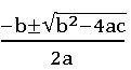
If α, β are the roots of the quadratic equation ax2 bx +c= 0, then α + β = -b/a and αβ = c/a.
Discriminate:
If ax2 + bx + c = 0 is a quadratic equation, then b2 – 4ac is called the discriminant of quadratic equation. b2 – 4ac is also the discriminant of quadratic expression ax2 + bx + c. It is denoted by ∆
∴ ∆ = b2 – 4 ac.
Nature of the roots:
The nature of the roots of the quadratic equation as follows:
- If ∆ > 0, then roots are real and distinct.
- If ∆ = 0, then roots are real and equal.
- If < 0, then roots are imaginary.
Note:
- If ∆ > 0 and b2 – 4 ac is a perfect square, then the roots are rational and distinct.
- If ∆ < 0 and b2 – 4 ac is not a perfect square, then the roots are irrational and distinct. Further, the roots are conjugate surds.
∎ If α, β are the roots of the quadratic equation ax2 + bx +c= 0, then ax2 + bx + c = a (x – α) (x – β)
∎ The quadratic equation whose roots are α, β is (x – α) (x – β) = 0 ⇒ x2 – (α + β) x + αβ = 0.
∎ The necessary and sufficient condition for the quadratic equations a1x2 + b1x + c1 = 0 and a2x2 + b2x + c2 = 0 to have common root is (c1a2 – c2a1)2 = (a1b2 – a2b1) (b1c2 – b2c1)
the common root is (c1a2 – c2a1)/ (a1b2 – a2b1).
∎ If f(x) = ax2 + bx +c= 0 is a quadratic equation then
- The quadratic equation whose roots are the reciprocals of the roots of f(x) = 0 is f(1/x) = 0.
- Whose roots are greater than by ‘k’ then those of f(x) = 0 is f (x – k) = 0.
- Whose roots are smaller by ‘k’ than those of f(x) = 0 is f (x + k) = 0.
- Whose roots are multiplied by ‘k’ of hose f(x) = 0 is f (x/k) = 0.
Sign of quadratic Expressions – change in signs:
∎ If the roots of quadratic equation ax2 + bx + c = 0 are complex roots, then for x ∈ R, ax2 + bx + c and ‘a’ have the same sign.
∎ If the roots of quadratic equation ax2 + bx + c = 0 are real and equal then for x ∈ R – {-b/2a}, ax2 + bx + c and ‘a’ have the same sign.
∎ Let α, β are the roots of the quadratic equation ax2 + bx +c= 0and α < β, then
- x ∈ R, α < x < β ⇒ ax2 + bx + c and ‘a’ have the opposite sign.
- x ∈ R, x < α or x> β ⇒ ax2 + bx + c and ‘a’ have the same sign.
Maximum and Minimum values:
Let f(x) = ax2 + bx +c is a quadratic expression then
- if a < 0, then f(x) has maximum value at x = -2b/a and maximum value is 4ac – b2/4a.
- if a > 0, then f(x) has minimum value at x = -2b/a and minimum value is 4ac – b2/4a.
Quadratic inequation:
A quadratic in equation in one variable is of the form ax2 + bx +c > 0 or ax2 + bx +c ≥ 0 or ax2 + bx +c< 0 or ax2 + bx +c ≤ 0 where a, b, c are real numbers and a ≠ 0. The values of x which satisfy given inequation are called the solution of the in equations.
⟹ Quadratic inequations are solved by two methods (i) Algebraic method (ii) Graphical method.
4.THEORY OF EQUATIONS
Polynomial: If n is non- negative integer and a0, a1, a2. …, an are real or complex numbers and a0 ≠ 0, then an expression
f(x) = a0 xn + a1 xn – 1+a2xn – 2 + … + an is called polynomial in x of degree n.
a0, a1, a2. …, an are called the coefficients of the polynomial f(x), a0 is called leading coefficient and an is called constant term.
Monic polynomial: A polynomial with leading coefficient is 1 is called a monic polynomial.
Remainder theorem: let f(x) be a polynomial of degree n> 0. Let a ∈C. Then there exist a polynomial q(x) of degree n – 1 such that
f(x) = (x – a) q(x) + f(a).
Factor theorem: let f(x) be a polynomial of degree n> 0. Let a ∈ C. We say that (x – a) is factor of f(x) if there exist a polynomial q(x) such that f(x) = (x – a) q(x).
⟹ let f(x) be a polynomial of degree n> 0, then (x – a) is factor of f(x) iff f(a) = 0.
The fundamental theorem of algebra: Every non-constant polynomial equation has at least one root.
⟹ The set of all roots of a polynomial f(x) = 0 of degree n> 0 is non-empty and has at most n elements. Also there exist α1, α 2. …, α n in C such that f(x) = a (x – α1) (x – α2) (x – α3) … (x – αn) where a is the leading coefficient of f(x).
The relations between the roots and the coefficients:
Let xn + p1 xn – 1+ p2xn – 2 + … + pn = 0 be a polynomial equation of degree n
Let α1, α 2. …, α n be roots.
xn + p1 xn – 1+ p2xn – 2 + … + pn = (x – α1) (x – α2) (x – α3) … (x – αn)
= xn – (α1+ α 2+ …+ α n) xn – 1+( α1 α 2+ α2 α 3 +…+ α n-1 α n) xn-2 – … (-1)n α1. α 2…. α n
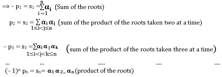
These equalities the relation between the roots and coefficient of the polynomial equation whose leading coefficient is 1.
Note:
1.For the quadratic equation: Let α, β be the roots of the quadratic equation ax2 + bx + c = 0, then
Sum of the roots = α + β = -b/a
Product of the roots = αβ = c/a
2.For the cubic equation: Let α, β and γ be the roots of the cubic equation ax3+ bx2 + cx + d = 0, then
Sum of the roots = α + β + γ = -b/a
Product of the roots taken two at a time= αβ + β γ + γ α = c/a
Product of the roots = αβ γ = -d/a
Notation: Let α, β and γ be the roots of a cubic polynomial, then
α + β + γ is denoted by ∑α, αβ + β γ + γ α is denoted by ∑ αβ , 1/α + 1/β + 1/γ is denoted by ∑1/α and α2 β + β2 α + α2 γ + γ2 β + β2 γ + γ2 α = ∑ α2 β + ∑ α β2
synthetic division: This method has two types
∗ Finding the quotient and remainder, when
a0 xn + a1 xn – 1+a2xn – 2 + … + an (a0 ≠ 0) is divided by (x – a).
∗ Finding the quotient and remainder, when
a0 xn + a1 xn – 1+a2xn – 2 + … + an (a0 ≠ 0) is divided by x2 – px – q.
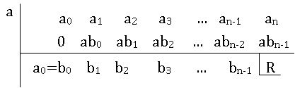
Method of finding the quotient and remainder, when a0 xn + a1 xn – 1+a2xn – 2 + … + an (a0 ≠ 0) is divided by (x – a)- (Horner’s Method):
The procedure of the above method:
- First write down the coefficients of xn, xn-1, …x, x0. If any term with xk (0 ≤ k < 1) is missing, take the coefficient of it as zero.
- Draw a vertical line to the left of ‘a0’ and write ‘a’ to the left of the vertical line on the same horizontal level as that of ‘a0’.
- Under a0 write 0 and draw the horizontal line below it. Below the horizontal line and below 0, write the sum a0 + 0 as the first term of the 3rd row, which is equal to b0 with a and write this product below a1 in the second row. The sum a1 + ab0 is b1. Write this in the 3rd row next to b0. Continue this process until the terms of the second and the third rows are filled.
- From the table, the quotient is b0 xn-1 + b1 xn – 2+ … + bn-1 and the remainder is R = an + abn-1.
Note:
- If the divisor is (x + a) then the above method can be used by replacing a with – a.
- If the divisor is ax – b, then replace a by b/a.
Method of finding the quotient and remainder, when a0 xn + a1 xn – 1+a2xn – 2 + … + an (a0 ≠ 0) is divided by x2 – px – q:
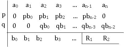
The procedure of the above method:
- First write down the coefficients of xn, xn-1, …x, x0. If any term with xk (0 ≤ k < 1) is missing, take the coefficient of it as zero.
- Draw a vertical line to the left of ‘a0’ and write p, q as column figures to the left of the vertical line in the second and third rows respectively. These are the negatives of the coefficient of x and the constant term in the divisor. Draw a horizontal line below the third row.
- Put 0 in two rows underneath a0 write this sum a0 + 0 + 0 as the first term of the 4th row, which is equal to b0. Next, multiply b0 with p and write this product below a1 and write the next column entry as 0. The sum a1 + pb0 + 0 is b1. Write this in the 4th row underneath a1 multiply b1 with p and b0 with q and write this product underneath a2. let the sum of a2, pb1 and qb0 be b2. continue this process until the terms an-1 are obtained. Name the 4th row under an-1 R1. below an put 0 and qbn-2 in the second and third rows respectively. Let the sum as an, 0 qbn-2 be R2. write it in the 4th row below an.
Trial and Error method: To find a root of f(x) = 0, we have to find out a value of x, for which f(x) = 0. Some times we can do this by inspection. This method is called trial and error method.
Multiple roots or repeated roots: let f(x) be a polynomial of degree n > 0. Let α1, α 2. …, α n be the roots of f(x) = 0 so that f(x) = a0 (x – α1) (x – α2) (x – α3) … (x – αn). A complex number α is said to be a root of f(x) = 0 of multiplicity m, if α = αk for exactly m values of k among 1,2, 3…, n. Roots of multiplicity m>1 are called multiple roots or repeated roots.
Roots of multiplicity 1 are called simple roots.
∎ Let f(x) be a polynomial of degree n> 0. Let α be a root of f(x) = 0 of multiplicity m. If m>1, then α is a root of the equation f’(x) = 0 of multiplicity m – 1. If m = 1, then f’(α) ≠ 0
∎ Let f(x) be a polynomial of degree n > 0. Let α be a root of f(x) = 0 of multiplicity m, then α is a root of the equation f(k)(x) = 0 of multiplicity m –k (k = 1, 2, 3, …, m – 1).
∎ Let f(x) be a polynomial of degree n> 0. Let α be a root of f(x) = 0 of multiplicity m Iff f(α) = f’(α) = … = f (m – 1) (α) and f(m)(α) ≠ 0.
Procedure to find multiple roots: Let f(x) be a polynomial. First, we find f’(x) and then find the HCF of f(x) and f’(x). Now we note that, if α is a root of the HCF of multiplicity k, then α is a multiple order of (k + 1) of f(x) =0.
∎ let f(x) be a polynomial with real coefficients. Let α ∈ C, then ![]()
∎ Let f(x) be a polynomial of degree n > 0, with real coefficients. Let a0 be the leading coefficient of f(x).
- If the equation f(x) = 0 has no real roots, then n is even and f(α), a0 have the same sign for all real values of α
- If n is odd, then the equation f(x) = 0 has at least one real root.
∎ Let f(x) be a polynomial of degree n > 0, with real coefficients. Let a and b be rational numbers, b > 0 and ![]() irrational. Then
irrational. Then ![]() is a root of f(x) = 0 if and only if another root is a
is a root of f(x) = 0 if and only if another root is a ![]() .
.
Roots with the change of sign:
If α1, α 2. …, α n are the roots of f(x) = 0, then -α1, – α 2. …, – α n are the roots of f(-x) = 0.
Roots multiplied by a given number:
If α1, α 2. …, α n are the roots of f(x) = 0, then for any non-zero complex number k, the roots of f(x/k) = 0 are kα1, k α 2. …, kα n.
Roots subtracted by a given number:
If α1, α 2. …, α n are the roots of f(x) = 0, then α1-h, α 2-h. …, – α n-h are the roots of f (x +h) = 0.
Roots added by a given number:
If α1, α 2. …, α n are the roots of f(x) = 0, then α1+h, α 2+h. …, – α n+h are the roots of f (x -h) = 0.
Reciprocal roots:
Let α1, α 2. …, α n are the roots of f(x) = 0. Suppose none of them non- zero, then 1/α1,1/ α 2. …,1/ α n are the roots of xn f (1/x) = 0.
∎ if α is a root of f(x) = 0, then α2 is a root of ![]()
Reciprocal equation:
Let f(x) be a polynomial of degree n > 0 is said to be reciprocal if f(0) ≠ 0 and ![]() ∀x ∈C-{0}, where a0 is the leading coefficient of f(x).
∀x ∈C-{0}, where a0 is the leading coefficient of f(x).
If f(x) is a reciprocal polynomial, then the equation f(x) = 0 is reciprocal equation.
∎ If f(x) = a0 xn + a1 xn – 1+a2xn – 2 + … + an be a polynomial of degree n > 0, then f(x) is reciprocal iff an – k = ak for k = 0, 1, 2,… , n or an – k = – ak for k = 0, 1, 2,… , n .
The reciprocal polynomial of class one and class two:
A reciprocal polynomial f(x) of degree n with leading coefficient a0 is said to be class one or class two according to as f(0) = a0 or –a0.
If f(x) is a reciprocal polynomial then the equation f(x) = 0 is said to be the reciprocal equation of class one or class two according to as f(x) is a reciprocal polynomial of class one or class two.
Note:
∎ For an odd degree, the reciprocal equation of class one -1 is the root and for an odd degree reciprocal equation of class two, 1 is root.
∎ For an even degree, the reciprocal equation of class two, – 1 and 1 roots.
∎ To solve the reciprocal equation of order 2m, divide the equation by xm and put x + 1/x = y or x – 1/x = y according to the equation of class one or class two. The degree of the transformed equation is m.
∎ For an odd degree reciprocal equation. To find the roots of it, divide f(x) by (x + 1) or (x – 1) according as the equation of class one or class two. Let Q(x) be the quotient obtained, then f(x) = (x+1) Q(x) or f(x) = (x – 1) Q(x) according as the equation of class one or class two and Q(x) is even degree reciprocal polynomial. The roots of Q(x) = 0 can be obtained by above procedure.
5.PERMUTATIONS AND COMBINATIONS
The fundamental principle of counting: if a work w1 can be performed in ‘m’ different ways and a second work w2 can be performed in ‘n ‘different ways, then the two works can be performed in ‘mn’ ways.
Permutation: From a given finite set of elements selecting some or all of them and arranging them in a line is called a ‘linear permutation’ or ‘permutation’.
Circular permutation
Permutations of ‘n’ dissimilar thing taken ‘r’ at a time:
∎ If n, r are positive integers and r ≤ n, then the no. of permutations of n dissimilar things taken as ‘r’ at a time is n (n – 1) (n – 2) (n – 3) … (n – r + 1).
Notation:
The number of permutations of n dissimilar things taken as r at a time is denoted by nPr or P (n, r) (1≤r≤n).
nPr = n (n – 1) (n – 2) (n – 3) … (n – r + 1)
∎ If n ≥1 and 0≤r≤n, then ![]()
nPn = n! and nP0 = 1.
∎ For 1≤r≤n , nPr = n. (n – 1) P (r – 1)
∎ If n, r are positive integers and 1 ≤r < n, then nPr = (n – 1) Pr + r. (n – 1) P (r – 1).
∎ The sum of all r-digit numbers that can be formed using the given ‘n’ non-zero digits (1 ≤r ≤n≤9) is
(n – 1) P (r – 1) × [ sum of the given digits × 1111… 1(r times)]
∎If ‘0’ is one digit among the given ‘digits, then we get that the sum of all r-digit numbers that can be formed using the given ‘n’ digits including ‘0’ is
{ (n – 1) P (r – 1) × [ sum of the given digits × 1111… 1(r times)]} – { (n – 2) P (r – 2) × [ sum of the given digits × 1111… 1((r-1) times)]}.
Note: If a set A has m elements and the set B has n elements, then the no. of injections into A to B is nPm if m ≤n and 0 if m> n.
Permutations when repetitions are allowed:
∎ Let n and r be positive integers. If the repetition of things is allowed, then the no. of permutations of ‘n’ dissimilar things taken ‘r’ at a time is nr.
Palindrome: A number or a word which reads the same either from left to right or right to left is called a palindrome.
Ex: 121, 1331, ATTA, AMMA etc.
Note: The no. of palindromes with r distinct letters that can be formed using given n distinct letters is
(i) nr/2 if r is even (ii) nr+1/2 if r is odd.
Circular permutation: From a given finite set of elements selecting some or all of them and arranging them around a circle is called a ‘circular permutation’.
∎ The no. of circular permutations of ‘n’ dissimilar things (taken all at a time) is (n – 1)!
∎ In case of the garlands of flowers, chains of beads etc, no. of circular permutations = ½ (n – 1)!
Permutations with constraint repetitions:
∎ The no. of linear permutations of ‘n’ things n which ‘p’ things are alike and the rest are different is ![]()
∎ The no. of linear permutations of ‘n’ things n which ‘p’ like things of one kind, q like things of the second kind, r like things of the third kind and the rest are different is 
Combinations:
A combination is only a selection. There is no importance to the order or arrangement of things in a combination.
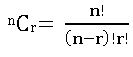
∎ The no. of combinations of ‘n’ dissimilar things taken ‘r’ at a time is denoted by nCr or C (n, r)
∎ 
∎ For 0≤r≤n, nCr = n C n – r
∎ If m, n are distinct positive integers, then the no, of ways of dividing (m + n) things into two groups containing m things and ‘n’ things is 
∎ If m, n, p are distinct positive integers, then the no, of ways of dividing (m + n + p) things into three groups containing m things, ‘n’ things and ‘p’ things is ![]()
∎ The no. of ways of dividing 2n dissimilar things into two equal groups containing ‘n’ things in each case is 
∎ The no. of ways of dividing ‘mn’ dissimilar things into m equal groups containing ‘n’ things in each case is ![]()
∎ The no. of ways of distributing ‘mn’ dissimilar things equally among m persons is 
• For 0 ≤ r, s ≤ n, if nCr = nCs then r =s or n = r + s.
• If 1 ≤ r ≤ n, then nCr-1 + nCr = (n+1) Cr.
• If 2 ≤ r ≤ n, then nCr-2 +2 nCr-1 = (n+2) Cr.
• If p things are alike of one kind, q things are alike of the second kind and r things are alike of the third kind, then the number of ways of selecting any no, of things out of these (p + q +r) things is (p + 1) (q+1)(r+1) – 1.
• The number of ways of selecting one or more things out of ‘n’ dissimilar things is 2n – 1.
• If p1, p2,…, pn are distinct primes and α1, α 2,…, α n are positive integers, then the number of positive divisors of ![]() is (α1+1)( α2+1) … (αk + 1).
is (α1+1)( α2+1) … (αk + 1).
Exponents of a prime in n! (n ∈ z+): Exponents of a prime number ‘p’ in n! is the largest integer ‘k’ such that pk divides n!
6.BINOMIAL THEOREM
Binomial: Binomial means two terms connected by either ‘+’ or ‘– ‘.
Binomial expansions:
(x + y)1 = x + y
(x + y)2 = x2 + 2xy + y2
(x + y)3 = x3 + 3x2 y + 3xy2 + y3 and so on, are called binomial expansions.
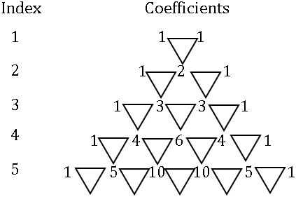
Binomial coefficients:
Coefficients of expansion (x + y) are 1, 1.
Coefficients of expansion (x + y)2 are 1, 2, 1
Coefficients of expansion (x + y) are 1, 3, 3, 1
And so on, are called binomial coefficients.
Pascal triangle:
Binomial theorem: Let n be a positive integer and x, a be real numbers, then
(x + a) n = nC0 xn a0 + nC1xn – 1 a1 + nC2 x n – 2 a2 +… + nCr xn – r ar + … + nCn x0 an
Note: –
Let n be a positive integer and x, a be real numbers, then
(i) (x + a) n = ∑ nCr xn – r ar
(ii) The expansion of (x + a) n has (n + 1) terms.
(iii) The rth term in the expansion of (x + a) n, which is denoted by Tr, is given by Tr = nCr-1 xn – r +1 ar-1 for 1≤ r≤ n + 1.
The general term of the binomial expansion:
In the expansion of (x + a)n, the (r + 1)th term is called the general term of the binomial expansion and it is given by Tr+1 = nCr xn –r ar for 0≤ r≤ n.
∎ (x – a) n = nC0 xn (-a)0 + nC1xn – 1 (-a)1 + nC2 x n – 2 (-a)2 +… + nCr xn – r (-a) r + … + nCn x0 (-a) n
= nC0 xn a0 – nC1xn – 1 a1 + nC2 x n – 2 a2 –… +(–1) r nCr xn – r ar + … + (–1) n nCn x0 an
And the general term is Tr+1 = (–1) r nCr xn –r ar for 0≤ r≤ n.
Trinomial Expansion: Let n ∈ N and a, b, c ∈ R, then (a + b + c) n can be expand using the binomial theorem taking a as the first term and (b + c) as the second term
(a + b + c) n = (a + (b+ c)) n = ∑ nC0 an-r (b + c) r (0≤ r≤ n)
⟹ no. of terms in the expansion of (a + b + c) n = ![]()
Middle terms in (x + a) n:
∎ if n is even then  term is the middle term.
∎ if n is odd then 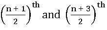 terms are the middle terms.
Binomial coefficients: The coefficients in the binomial expansion (x + a) n are nC0, nC1, …, nCr, …, nCn these coefficients are called binomial coefficients. When n is fixed these coefficients are denoted by C0, C1, …, Cr, …, Cn. respectively.
Note:
- The binomial expansion of (1 + x) n = nC0 + nC1x + nC2 x 2 +… + nCn xn. This expansion is called the standard binomial expansion.
With the standard notation, if n is a positive integer, then
- C0 + C1 + C2 …+ Cn = 2n
- C0 + C2 + C4 …+ Cn = 2n-1 if n is even
- C0 + C2 + C4 …+ Cn-1 = 2n-1 if n is odd
- C1 + C3 + C5 …+ Cn-1 = 2n-1 if n is even
- C1 + C3 + C5 …+ Cn = 2n-1 if n is odd
Integral part and Fractional part: If x is any real number, then there exist an integer n such that n ≤ x < n+ 1. This integer n is called an integral part of the real number x and it is denoted by [x]. The real number x – [x] is called fractional part of x and it is denoted by {x}.
Numerically greatest term: In the binomial expansion of (1 + x) n, the rth term Tr is called numerically greatest term if, ![]()
⟹ if ![]() = p, where p is a positive integer then, pth and (p + 1)th are the numerically greatest terms.
= p, where p is a positive integer then, pth and (p + 1)th are the numerically greatest terms.
⟹ if ![]() = p + F, where p is a positive integer and 0 < F < 1 then, (p + 1)th is the numerically greatest term.
= p + F, where p is a positive integer and 0 < F < 1 then, (p + 1)th is the numerically greatest term.
⟹ To find the numerically greatest term(s) in the binomial expansion of (a + x)n we write (a + x)n = an(1 + x/a)n and then find the numerically greatest term(s) by using above rules.
Largest Binomial coefficient:
The largest binomial coefficient(s) among nC0, nC1, …, nCr, …, nCn is (are)
(i) ![]() if n is even integer.
if n is even integer.
(ii) 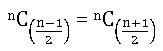 if n is an odd integer
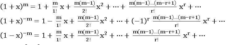
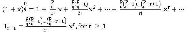
Binomial theorem for Rational Index:
If m is a rational number and x is a real number such that – 1 < x < 1, then
Rational Index: –

7. PARTIAL FRACTIONS
Rational fraction: If f(x) and g(x) are two polynomials and g(x) is a non-zero polynomial, then![]() is called a rational fraction or polynomial fraction or simply a fraction.
is called a rational fraction or polynomial fraction or simply a fraction.
Ex:![]()
Proper and Improper Fractions: A rational fraction![]() is called a Proper fraction if the degree of f(x) is less than the degree of g(x). Otherwise, it is called an improper fraction.
is called a Proper fraction if the degree of f(x) is less than the degree of g(x). Otherwise, it is called an improper fraction.
Ex:  is a proper fraction and
 is an Improper fraction.
Irreducible Polynomial: A polynomial f(x) is said to be irreducible if it can not be express as a product of two polynomials g(x) and h(x) such that the degree of each polynomial is less than the degree of f(x). If f(x)is not irreducible then we say that f(x) is reducible.
Ex: 3x – 1, x2 + x + 1 are irreducible polynomials.
Division Algorithm for Polynomials: If f(x) and g(x) are two polynomials with g(x) ≠ 0, then there exist unique polynomials q(x) and r(x) such that f(x) = q(x) g(x) + r(x) , where either r(x) = 0 or the degree of r(x) is less than the degree of g(x).
Partial Fraction: If a proper fraction is expressed as the sum of two or more proper fractions, wherein the power of the denominator of irreducible polynomials, then each proper fraction in the sum is called a partial fraction of the given fraction.
∎ Partial Fraction of  when g(x) contains linear factors:
Rule – 1: Let ![]() be a proper fraction. To each non- repeated factor of g(x), there will be a partial fraction of the form
be a proper fraction. To each non- repeated factor of g(x), there will be a partial fraction of the form![]() where A is a non-zero real number, to be determined.
where A is a non-zero real number, to be determined.
Rule – 2: Let ![]() be a proper fraction. To each factor (ax + b)n, a ≠ 0 where ‘n’ is a positive integer, of g(x) there will be a partial fraction of the form
be a proper fraction. To each factor (ax + b)n, a ≠ 0 where ‘n’ is a positive integer, of g(x) there will be a partial fraction of the form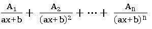 where A1, A2, …, An are to be determined constants. Note that An ≠ 0 and Rule –1 is a particular case of Rule-2 for n = 1.
∎ Partial Fraction of when g(x) contains irreducible factors:
Rule – 3: Let – be a proper fraction. To each non- repeated quadratic factor (ax2 + bx + c), a ≠ 0 of g(x) there will be a partial fraction of the form![]() where A, B are real numbers, to be determined.
where A, B are real numbers, to be determined.
Rule – 4: Let – be a proper fraction. If n (>1)∈ N is the largest exponent so that (ax2 + bx + c)n, a ≠ 0) factor of g(x) there will be a partial fraction of the form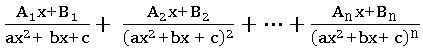 where A1, A2, …, An and B1, B2, …, Bn are real numbers, to be determined.
Partial Fraction of when is an Improper fraction:
Case (1): If degree f(x) = degree of g(x) then by division algorithm there exist a unique constant k and r(x) such that f(x) = k g(x) + r(x), where either r(x) = 0 or the degree of r(x) is less than the degree of g(x) and the constant k is the quotient of the coefficient of the highest degree terms of f(x) and g(x).
![]() can be expressed as k +
can be expressed as k + ![]() where
where![]() is a proper fraction which can be resolved into a partial fraction using the above rules.
is a proper fraction which can be resolved into a partial fraction using the above rules.
Case (2): If degree f(x) > degree of g(x) then by division algorithm![]() can be expressed as q(x) +
can be expressed as q(x) + ![]() where q(x) is a non-zero polynomial and
where q(x) is a non-zero polynomial and ![]() is a proper fraction which can be resolved into a partial fraction using above rules.
is a proper fraction which can be resolved into a partial fraction using above rules.
8. MEASURES OF DISPERSION
The measure of dispersion: In a measure of central tendency, we have to know a measure to describe the variability. This method is called a measure of dispersion.
Measuring dispersion of a data is significant because it determines the reliability of an average by pointing out as to how far an average is representative of the entire data.
Some measures of dispersion are: (i) Range (ii) Mean deviation (iii) Standard deviation
Range:
For ungrouped data, the range is the difference between the maximum and minimum value of the series of observations.
For grouped data range is approximated as the difference between the upper limit of the largest class and the lower limit of the smallest class.
Mean deviation:
To find the dispersion of values of x from a central value ‘a’ we find the deviation about ‘a’. They are (x – a)’s. To find the mean deviation we have to sum up all such deviations.

Mean deviation from the mean for ungrouped data:
Let x1, x2, …, xn be n observations of discrete data.
Steps for finding the Mean deviation from the mean for ungrouped data:
- First, we have to find the mean (
 ) of the n observations. Let it be ‘a’
 - Find the deviations of each xi from ‘a’, i.e., x1 – a, x2 – a, …, xn – a.
- Find the absolute values of i.e., of these deviations by ignoring the negative sign, if any, in the deviation computed in step 2.
- Find the arithmetic mean of the absolute values of the deviations.
M.D from the mean =
Mean deviation from the median for ungrouped data:
Let x1, x2, …, xn be n observations of discrete data.
Steps for finding the Mean deviation from the median for ungrouped data:
- First, we have to find the median of the n observations. Let it be ‘a’
- Find the deviations of each xi from ‘a’, i.e., x1 – a, x2 – a, …, xn – a.
- Find the absolute values of i.e.,
 of these deviations by ignoring the negative sign, if any, in the deviation computed in step 2.
 - Find their arithmetic mean as M.D from median =

Mean deviation for a grouped data:
A data can be arranged or grouped as a frequency distribution in two ways: (i) Discrete frequency distribution and (ii) Continuous frequency distribution.
(i) Discrete frequency distribution:
If x1, x2, …, xn are of ‘n’ observations occurring with frequencies f1, f2, …, fn Then we can represent this data in the following manner:
| xi | x1 | x2 | x3 | … | xn |
| fi | f1 | f2 | f3 | … | fn |
This form is called the discrete frequency distribution
Mean deviation about the mean and median:
Mean = ![]()
M.D(mean) =![]()
M.D(median) =![]()
Where N is total frequency.
(ii) Continuous frequency distribution: –
Continuous distribution is a series in which the data is classified into different class-intervals along with their respective frequencies.
Mean deviation about the means and median:
Mean = ![]()
M.D(mean) =![]()
Median = 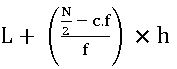
M.D(median) =![]()
Where N is total frequency.
Step- Deviation method: If the midpoints of the class intervals xi as well as their associated frequencies are very large then we use this method.
Arithmetic mean = ![]()
Where ![]()
Variance and Standard Deviation of un grouped data:
If x1, x2, …, xn are n observations and is their mean, then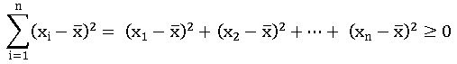
We have the following cases:
Case(i): if ![]() = 0, then each
= 0, then each![]() = 0 which implies all observations are equal to the mean and there is no dispersion.
= 0 which implies all observations are equal to the mean and there is no dispersion.
Case(ii): if ![]() is small, then it indicates that each observation xi is very close to the mean and hence the degree of dispersion is low.
is small, then it indicates that each observation xi is very close to the mean and hence the degree of dispersion is low.
Case(iii): if ![]() is larger, then it indicates the higher degree of dispersion of the observations from the mean .
is larger, then it indicates the higher degree of dispersion of the observations from the mean .
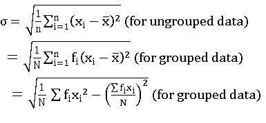
Variance = σ2= ![]()
Standard deviation
∎ The coefficient of variation of a distribution (C.V.) =![]()
9. PROBABILITY
Random Experiment: If the result of an experiment is not certain and is any one of the several possible outcomes, then the experiment is called ‘random experiment.
Sample space: The set of all possible outcomes of an experiment is called ample space when ever the experiment conducted and is denoted by ‘S’.
Event: Any subset of the sample space is called an event.
Complimentary of an event: The complementary of an event E , is denoted by Ec , is the event given by Ec = S – E which is called the complimentary event of E.
Equally likely events: two events are said to be equally likely events when chance of occurrence of one event is equal to that of other.
Exhaustive events: A set of events is said to be exhaustive if the performance of the experiment always result in the occurrence of the at least one of them.
The events E1, E2, …, En are said to be exhaustive if E1∪ E2∪…, ∪ En = S.
Mutually Exclusive events: A set of events is said to be mutually exclusive if happening of one of them prevents the happening of any one of remaining events.
The events E1, E2, …, En are said to be exhaustive if Ei ∩ Ej =∅ for i ≠ j, 1 ≤i, j≤ n.
Classical definition of Probability: In a random experiment, let there be n mutually exclusive, exhaustive and equally likely events.
E be the event of the experiment. ‘m’ elementary events are favourable to an event E, then the probability of E is defined as P (E) =![]()
For any event E, 0 ≤ P(E) ≤1.
∎ If Ec is the non-occurrence of E, then the probability of on-occurrence of E is P (Ec)
P (Ec) = 1 – P (E) ⇒ P (Ec) + P (E) = 1
Limitations of the Classical definition of the probability:
- If the out comes of the random experiment are not equally likely, then the probability of an event in such experiment is not defined.
- If the random experiment contains infinitely many out comes, then his definition cannot be applied to find the probability of an event in such an experiment.
Relative frequency (Statistical or Emperical) definition probability:
Suppose a random experiment is repeated n times, out of which an event E occurs m(n) times, then the ratio ![]() is called the nth relative frequency of the event E.
is called the nth relative frequency of the event E.
Let r1, r2, …, rn be the sequence. If rn tends to a definite limit,![]() , l is defined to be the probability of the event E and we write P (E) =
, l is defined to be the probability of the event E and we write P (E) = ![]()
Deficiencies of the relative frequency definition of probability:
- Repeating a random experiment infinitely many times is practically impossible.
- The sequence of relative frequencies is assumed to tend to a definite limit, which may not exist.
- The values r1, r2, …, rn are not real variables. Therefore, it is not possible to prove the existence and the uniqueness of the limit of rn as n → ∞, by applying methods used in calculus.
Probability Function:
Let S be the sample space of a random experiment, which is finite. Then a function P: S → R satisfying the following axioms is called a Probability function.
(i) P (E) ≥ 0 ∀ E ∈ S (axiom of non-negativity)
(ii) P (S) = 1 (axiom of certainty).
(iii) If E1, E2 ∈ S and E1 ∩ E2 =∅, then P (E1 ∪ E2) = P (E1) + P (E2) (axiom of additivity).
For each E ∈ S, the real number P (E) s called the probability of the event E. If E = {a}, then we write p(a) instead of P ({a}).
Note:
- P (∅) = 0 for any sample space S, S ∪ ∅ = S and S∩ ∅ = ∅. P (S) = (S ∪ ∅) = P (S) + P (∅) = P (S) (∵ P (∅) = 0).
- If S is countably infinite, then axiom (iii) of the above definition is to be replaced by (iii)*: if
 is a sequence of pairwise mutually exclusive events, then
- Suppose S be a sample space of a random experiment. Let P be a probability function. If E1, E2, …, En are finitely many pairwise mutually exclusive events, then P (E1∪ E2∪…, ∪ En) = P (E1) + P (E2) + … + P (En)
⟹ If E1, E2 are any two events in a sample space S, then
Addition theorem on probability: If E1, E2 are any two events in a sample space S and P is a probability function, then P (E1∪ E2) = P (E1) + P (E2) – P (E1∩ E2)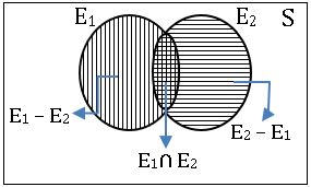
P (E1 – E2) = P (E1) – P (E1∩ E2)
P (E2 – E1) = P (E2) – P (E1∩ E2)
Set – theoretic descriptions:
| Event | Set-theoretic description |
| Event A or Event B to occur | A∪B |
| Both event A and B occur | A∩B |
| Neither A nor B occur | (A∪B) c = Ac ∩ Bc |
| A occurs but B does not occur | A ∩ Bc or A\B |
| Exactly one of the event A, B to occur | (A∩B) c ∪ (Ac ∩ B) or (A – B) ∪ (B – A) or (A∪B) – (A ∩ B) |
| Not more than one of the events A, B occurs | (A∩B) c ∪ (Ac ∩ B) ∪ (Ac ∩ Bc) |
| Event B occurs whenever event A occurs | A ⊆ B |
Conditional event: If A, B are two events of random experiment, then the event of happening (occurring) B after the event A happens(occurs) is called conditional event. It is denoted by B\A.
Conditional probability: If A, B are two events and P (A) ≠ 0, then the probability of B after the event A has occurred is called conditional probability. It is denoted by P (B/A) and is defined by P(B/A) = ![]()
Multiplication theorem of probability: If A, B are two events of random experiment with P (A) > 0 and P (B) > 0, then P (A∩B) = P (A) P (B/A) = P (B) P (A/B).
⟹ Two events A and B said to be independent if P (B/A) = P(B) or P (A/B) = P (A)
⟹ Two events A and B said to be independent if P (A∩B) = P (A). P (B)
⟹ The events A1, A2, …, An are said to be independent if P (A1∩ A2∩ …∩ An) = P (A1). PA2). …. P(An).
Bayes Theorem:
If A1, A2, …, An are mutually exclusive and exhaustive events in a sample space S such that P (Ai) > 0 for i = 1, 2, 3, …, n and E is an event with P (E) > 0, then

10. RANDOM VARIABLES AND PROBABILITY DISTRIBUTIONS
Random variable: Let S be a sample space of a random experiment. A real valued function X: S → R is called random variable.
∎ A set A is said to be countable if there exist a bijection from A into a subset of N.
Probability distribution Function: If X: S → R is a random variable connected with a random experiment and P is a probability function associate with it. The unction F: R → R defined by F(x) = P (X ≤ x) is called probability distribution function of the random variable X.
Discrete or discontinuous Random variable: Let S be a sample space, a random variable X: S → R is said to be Discrete or discontinuous if the range of X is countable.
I.POBABILITY DISTRIBUTION:
If X: S → R is a discrete random variable with range {x1, x2, x3………}, then {P(X = xr; r = 1, 2, 3, …, n} is called probability distribution of X.
The table for the probability distribution of the discrete random variable X is:
| X = xi | x1 | x2 | x3 | … | xn |
| P (X = xi) | P (x1) | P (x2) | P (x3) | … | P (xn) |
Mean (μ) =∑xi P (X = xi)
Variance = σ2 = ∑ (xi – μ)2 P (X = xi) = ∑ xi2 P (X = xi) – μ2
Standard deviation is σ.
II.BINOMIAL or BERNOULLI DISTRIBUTION:
Let n be a positive integer and p be the random number such that 0 < p < 1. A random variable X with range {0, 1, 2, 3, …, n} is said to have a Binomial distribution with parameters n and p, if
P (X = x) = nCx px qn – x for x = 0, 1, 2, …, n and q = 1 – p.
Mean = np
Variance = npq.
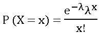
III. POISSON DISTRIBUTION:
Let λ > 0 be a real number. A random variable X with range {1, 2, 3, …, n} is said to be Poisson distribution with parameter λ if,
Mean = λ
Variance = λ
Poisson distribution as a limiting form of Binomial distribution:
Poisson distribution can be derived as the limiting case of binomial distribution in the following case.
If λ > 0 for each positive integer n > λ, let Xn be the Binomial variable B (n, λ/n). using the fact that ![]() we can prove that for every non-negative integer k,
we can prove that for every non-negative integer k,![]()
My App: Click Here
Visit My Youtube Channel: Click on below logo