
viii Class Maths || TS 8th Class Maths Concept
viii Class Maths
- TS 6th Maths Concept
- TS 7th Maths Concept
- TS 8th Maths Concept
- TS 9th Maths Concept
- TS 10th Maths Concept
viii Class Maths
Studying maths in VIII class successfully meaning that children take responsibility for their own learning and learn to apply the concepts to solve problems.
This notes is designed by the ‘Basics in Maths team’. These notes to do help students fall in love with mathematics and overcome fear.
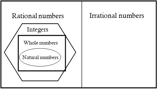
1. RATIONAL NUMBERS
• Natural numbers: All the counting numbers starting from 1 are called Natural numbers.
1, 2, 3… Etc.
• Whole numbers: Whole numbers are the collection of natural numbers.
0, 1, 2, 3 …
• Integers: integers are the collection of whole numbers and negative numbers.
….., -3, -2, -1, 0, 1, 2, 3….
• Rational numbers: The numbers which are written in the form of p/q, where p, q are integers and q ≠ 0 are called rational numbers. Rational numbers are denoted by Q.
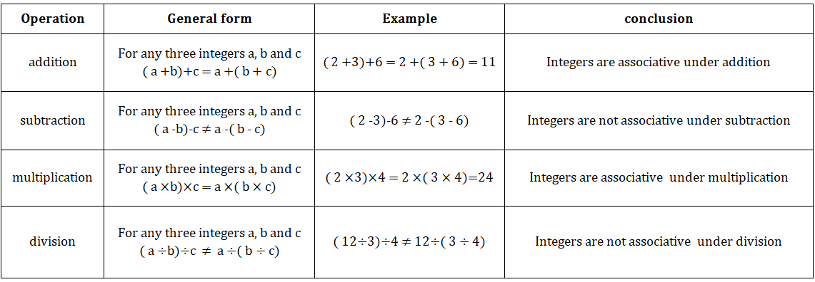
Properties of Rational numbers
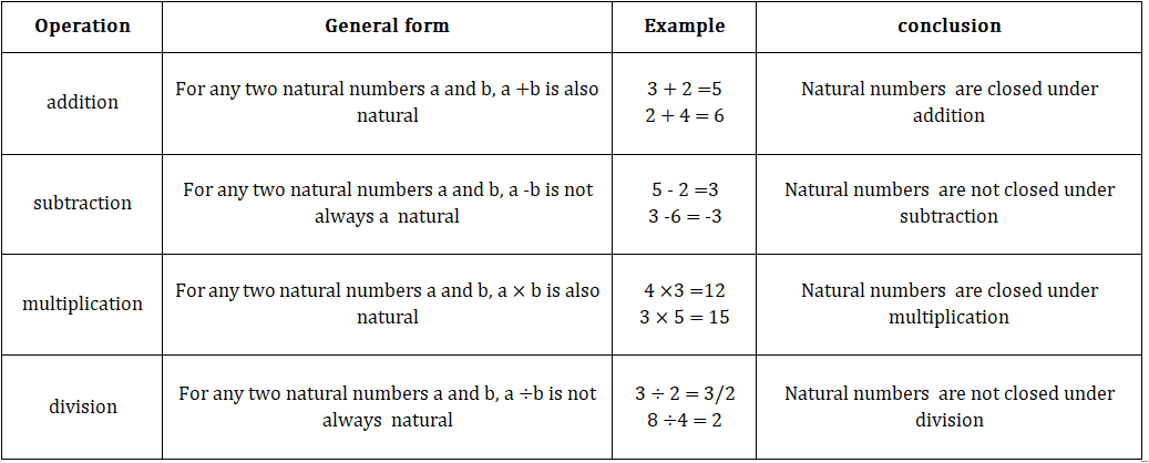
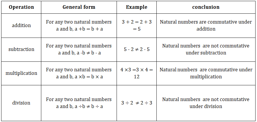
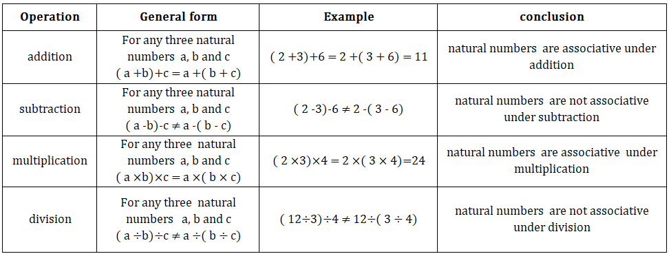
• Natural numbers:
1.Closure property:-
2.Commutative property:-
3. Associative property:-
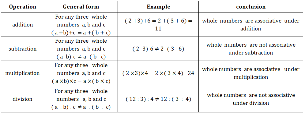
• Whole numbers:
1. Closure property:-
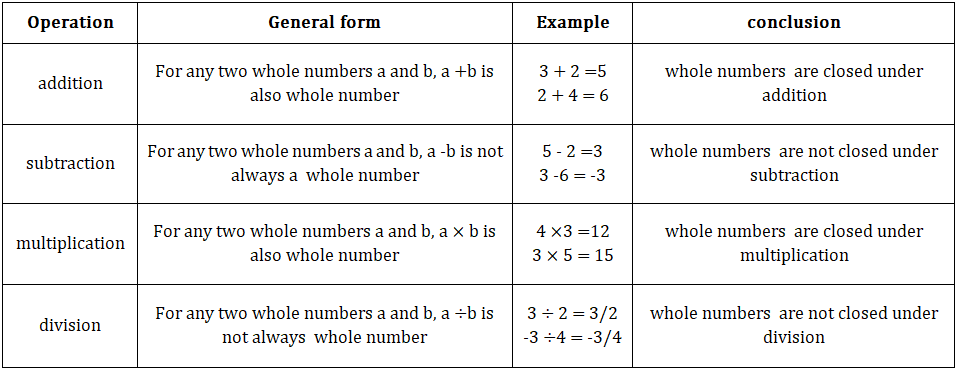
2.Commutative property:-
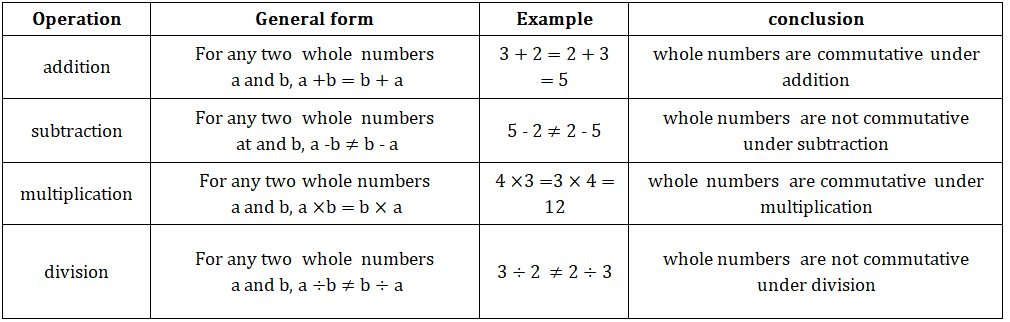
3. Associative property:-
• Integers:
1. Closure property:-
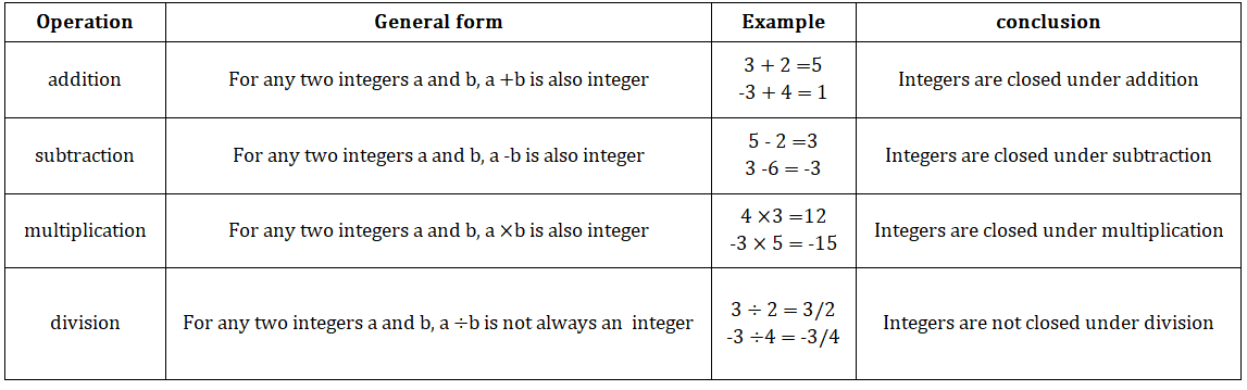
2.Commutative property:-
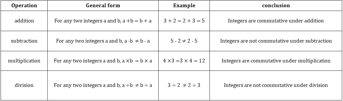
3. Associative property:-
• Rational numbers:
1. Closure property:-
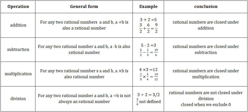
2.Commutative property:-
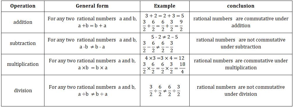
3. Associative property:-

Additive identity:-
1 + 0 = 0 + 1 = 1, 3/2 + 0 = 0 + 3/2 = 3/2
• For any rational number ‘a’, a + 0 = 0 + a
• 0 is the additive identity.
Additive inverse:-
2 + (-2) = (-2) + 2 = 0, 5 + (-5) = (-5) + 5 = 0
• For any rational number ‘a’, a+ (-a) = (-a) + a = 0
• Additive inverse of a = -a and additive inverse of (-a) = a
Multiplicative identity:-
2 × 1 = 1 × 2 = 2, 6 ×1/6 = 1 × 1/6 = 1/6
• For any rational number ‘a’, a × 1 = 1 × a = a
• 1 is the multiplicative identity.
Multiplicative inverse:-
2 × 1/2 = 1/2 × 2 =1
For any rational number ‘a’,
a × 1/a = 1/a × a = 1
• multiplicative inverse of a =1/a
• Multiplicative inverse of 1/a= a.
Distributive property:-
For any three rational numbers a, b and c,
a × (b + c) = (a × b) + (a × c)
3/2×(5/3+1/5)=(3/2×5/3)+(3/2×1/5)
Representing rational numbers on a number line:
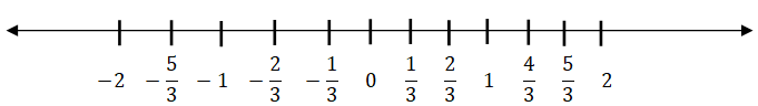
Ex: represent 29/6 on a number line
![]() this lies between 4 and 5
this lies between 4 and 5
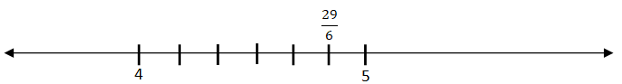
Divide the number line between 4 and 5 into 6 equal parts. Mark 5th part counting from 4.
The role of zero:
• If 0 is added to any rational number, then the rational number remains the same.
For any rational number ‘a’ a + 0 = a = 0 + a
• 0 is the additive identity.
• Natural numbers do not have an additive identity.
Additive inverse:-
for any rational number ‘a’
a + (-a) = 0 = (-a) + a
3 + (-3) = 0, 10 + (-10) = 0
• additive inverse of ‘a’ is ‘-a’ and additive inverse of ‘-a’ is ‘a’
The role of 1:
• If 1 is multiplied to any rational number, then the rational number remains same.
For any rational number ‘a’ a × 1 = a = 1 × a
- 1 is the multiplicative identity.
Multiplicative inverse:-
3 × 1/3 = 1 = 1/3 × 3
for any natural number ‘a’
a × 1/a = 1 = 1/a ×a
• Multiplicative inverse of ‘a’ is ‘1/a’ and multiplicative inverse of ‘1/a’ is ‘a’
Distributive property:
For any 3 rational numbers a, b and c, a (b + c) = ab + ac
Ex:- 1/3 (2/5 + 1/5) = 1/3(3/5) = 3/15
1/3× 2/5 + 1/3 × 1/5 = 2/5 + 1/5 = 3/5
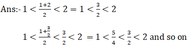
Inserting rational numbers between given two numbers:
• There are infinitely many rational numbers between given two numbers.
• We have two methods to find rational numbers between two numbers.
First method: – First we have to convert given rational numbers as the same denominator and write the rational numbers which come between given numbers.
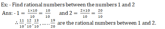
Second method: – if a and b any given rational numbers then a/bis a rational number between a and b.
The decimal representation of rational numbers
The decimal expansion of rational is either terminating or non-terminating repeating decimal.
Note:-Decimal numbers with the finite no. of digits is called terminating Decimal numbers with the infinite no. of digits is called non-terminating decimal. In a decimal, a digit or a sequence of digits in the decimal part keeps repeating itself infinitely. Such decimals are called non-terminating repeating decimals.
Terminating decimals:
Consider a rational number ![]()
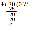
![]() = 0.75
= 0.75
Non-terminating decimals:
Consider a rational number 2-3
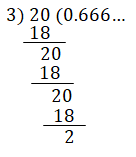
2/3 = 0.66666…
2/3 = ![]()
2. LINEAR EQUATIONS IN ONE VARIABLE
Equations: An algebraic equation is the equality of algebraic expressions involving variables and constants.
- It has an equality sign.
- The expression on the left of the equality sign is called the LHS (Left Hand Side) and right of the equality is called RHS (Right Hand Side) of the equation.
- In an equation, the value of RHS and LHS are equal. This happens to be true only for certain values of the variable. This value is called the solution of the equation.
Linear equations: If the degree of the equation is 1, then it is called a linear equation.
Ex: 2x – 3 = 5, x = 3y, 5x + 3y = 3 and so on.
Simple equations or linear equations in one variable: An equation of the form ax + b = 0 or ax = b where a, b are constants and a≠0is called a linear equation in one variable or simple equation.
Ex: 2x + 3 = 7, x = 3, 2 – 3x = – 1 and so on.
Note: if we transpose terms from LHS to RHS or RHS to LHS
‘+’ quantity becomes ‘– ‘quantity
‘–’ quantity becomes ‘+ ‘quantity
‘×’ quantity becomes ‘÷ ‘quantity
‘÷’ quantity becomes ‘× ‘quantity
Solving simple equation having the variable on one side:
Ex: solve the equation 2x + 32 = 2
Sol: 2x = 2 – 32 (transpose 32 to RHS)
2x = – 30
x = – 30/2 (transposing to RHS)
∴ solution of 2x + 32 = 2 is – 10.
Solving simple equation having the variables on both sides:
Ex: solve the equation 9y + 5 = 15y – 1
Sol: given equation is 9y + 5 = 15y – 1
9y – 15y = – 1 – 5 (Transposing 5 to RHS and 15y to LHS)
–6y = – 6
y = –6/–6 = 1
y = 1
∴ solution of the equation 9y + 5 = 15y – 1 is 1.
Method of cross Multiplication:
![]() = ad = bc
= ad = bc
Multiply the numerator of the LHS by the denominator of the RHS and multiply the numerator of the RHS by the denominator of LHS. This method is called the cross multiplication method.
Reducing Equations to simpler form – Equations Reducible to Linear form:
Ex: solve the equation ![]()
Sol: given equation is ![]()
⇒ 7(5x + 2) = 12(2x + 3) (∵ by cross multiplication method)
⇒ 35x + 14 = 24x + 36
⇒ 35x – 24x = 36 – 14 (by transposing terms)
⇒ 11x = 22
∴ x = 2 is the solution of given equation.
viii Class Mathsviii Class Maths
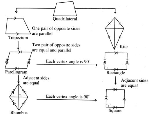
3.CONSTRUCTION OF QUADRILATERALS
Quadrilateral: A closed figure with four sides is called a quadrilateral.
It has 4 sides, 4 vertices, 4 angles and two diagonals.
Types of quadrilaterals:
1.Trapezium: A quadrilateral with at least one pair of parallel sides is called a trapezium.
Opposite sides are not equal and diagonals are not equal
2.Parallelogram: A quadrilateral with two pairs of opposite sides are parallel is called a parallelogram.
Opposite sides are parallel and equal
Opposite angles are equal
Diagonals are not equal.
Diagonals bisect each other.
3.Rectangle: A parallelogram with one of the angles 900 is called a rectangle.
Opposite sides are parallel and equal
Opposite angles are equal
Diagonals are equal.
Diagonals bisects each other.
4.Rhombus: A parallelogram with adjacent sides are equal is called rhombus.
All sides are equal
Opposite angles are equal
Diagonals are not equal.
Diagonals bisect each other and angle between diagonals is 900
5.Square: A rhombus with four right angles is called a square.
All sides are equal
Opposite angles are equal
Diagonals are equal.
Diagonals bisect each other and angle between diagonals is 900
6.Kite: A quadrilateral with two pairs of adjacent sides is called a kite.
Constructing a Quadrilateral:
We can draw quadrilaterals when the following measurements are given.
- When 4 sides and one angle are given
- When 4 sides and one diagonal are given
- When three sides and two diagonals are given
- When two adjacent sides are given and three angles are given
- When three side and two included angles are given
Type of Quadrilateral – No, of individual measurements:
| Type of quadrilateral | No. of individual measurements |
| Quadrilateral | 5 |
| Trapezium | 4 |
| Parallelogram | 3 |
| Rectangle | 3 |
| Rhombus | 2 |
| Square | 1 |
Example 1:
Construct the quadrilateral PQRS with the measurements: PQ = 5.5cm, QR = 3.5 cm, RS= 4 cm, PS = 5 cm and ∠P = 450.
Steps of construction: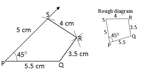
- Construct a line segment PQ with a radius 5.5cm.
- With the center, P draw a ray and an arc that are equal to 450 and 5 cm.
- These intersecting points are kept as S.
- With centers S, Q draws two arcs equal to Radius 4 cm, 3.5 cm respectively.
- The intersecting point of these two arcs is kept as R.
- Join Q, R, and S, R
- Therefore, the required quadrilateral PQRS formed.
Example 2
Construct the parallelogram PQRS with the measurements: PQ = 4.5cm, QR = 3 cm and ∠PQR = 600
In parallelogram PQRS with the measurements: PQ = 4.5cm, QR = 3 cm and ∠PQR = 600
⇒ RS = 4.5cm, PS = 3 cm (in a parallelogram opposite sides are equal)
Steps of construction 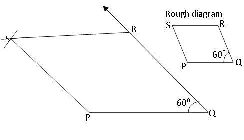
- Construct a line segment PQ with a radius 4.5cm.
- With the center, Q draws a ray and an arc that are equal to 450 and 3 cm.
- These intersecting points are kept as R.
- With centers R, P draws two arcs equal to radius 4 cm, 3.5 cm respectively.
- The intersecting point of these two arcs is kept as S.
- Join P, S and R, S
- Therefore, the required parallelogram PQRS formed.
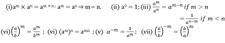
4. EXPONENTS AND POWERS
We know that a2 = a × a (two times)
a3 = a × a × a (three times)
⇒ a × a × a × a × a … m times = am
Here, am is called the exponent form.
- In exponent, form am, ‘a’ is base, ‘m’ is exponent, power, or index.
- We read am as a raised to the power of m.
Laws of exponents:
Express small numbers in Standard form by using exponents:
- If a number is expressed in the form of m ×10n where 1≤m<10, n is any integer, then that number is in standard form.
- Very small numbers can be expressed in standard form using negative exponents.
Ex: express 0.0000456 in standard form
Sol : 0.0000456 = 456/10000000 = 456/107 = 456 × 10-7.
5. COMPARING QUANTITIES USING PROPORTION
Ratio: comparing two quantities of the same kind by using division is called ratio.
Ratio of two quantities a and b is denoted by a: b.
Per cent: percent means ‘per hundred’ or out of hundred’. The symbol % stands for percent.
Discount:
Marked price (M.P): – The price printed on an article by the manufacturer is called the marked price. It is also called as list price or usual price or catalog price.
Discount: – Discount is the reduced marked price. It is generally given as a percent of the marked price. Discount is always depending on the marked price.
The net price or selling price: – The difference between the M.P. and discount is called net price or selling price.
Example: A TV is marked at ₹ 18000 and the discount allowed on it is 10%. What is the amount of discount and its sale price?
Ans: Given marked price = ₹18000, discount percentage = 10%
Now, discount = 10% 0f 18000 = ![]() = 1800
= 1800
Selling price = marked price – discount = 18000 – 1800 = 16200.
∴ selling price = ₹ 16,200.
Profit and loss:
Cost price (C.P.): – Cost price is the price for which an article is bought or the price paid by a customer to by an article.
Selling price (S.P.): – Selling price is the price for which an article is sold.
Profit: – If the Selling price is greater than the cost price, then we get the profit.
Profit = S.P – C.P.
Loss: – If the Selling price is less than the Cost price then, we get a loss.
Loss = C.P – S.P.
Some formulae in profit and loss:
![]()
For-Profit:
![]()
For Loss:
![]()
Sales tax/Value added tax:
The government collects taxes on every sale. This is called VAT. Shop keeper collects this from the customers and pays it to the Govt.
VAT is changed on the Selling price of an item and will be included in the bill. VAT is an increased percent of the selling price.
Example:
The cost of an article is ₹ 500. The sales tax is 5%. Find the bill amount.
Ans: cost price of an article = ₹500
% of Sales tax = 5
Sales tax paid = ₹
Bill amount = cost price + sales tax paid
= 500 + 25
= ₹ 525.
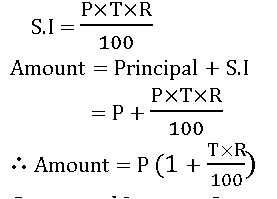
Simple interest:
Principal: – The money which is borrowed is called ‘principal’.
Rate of interest: – the percentage of interest per year is called the rate of interest.
Time: – The period for which money is called time.
Interest: – The money which is paid for the use of the principal is called interest.
Amount: – The total money which is paid after the expiry of the time is called the amount.
Compound Interest: Compound interest allows us to earn interest on interest.
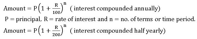
- The time period after which interest is added to the principal is called the conversion period. When interest is compounded h yearly, there are two conversion periods in a year. In such case, half-year rate will be half of the annual rate.
6. SQUARE ROOTS AND CUBE ROOTS
Square: Square number is the number raised to power 2. The number is obtained by the number multiplied by itself.
- If a natural number p can be expressed as q2, where q is also natural, then p is called a square number.
Ex: – 1) square of 9 = 92 = 9× 9 = 18, 2) square of 4 = 42 = 4× 4
Perfect Square: A natural number is called a perfect square if it is the square of some natural number.
Ex: – 1,4,9, …etc.
Properties of perfect square:
- The square of even numbers is always an even number.
Ex: – 22 = 4 (4 is even), 62 = 36 (36 is even), here 2, 6 are an even number.
- The square of an odd number is always an add number.
Ex: – 32 = 9 (9 is even), 152 = 225 (225 is even), here 3, 15 are an odd number.
- The square of a proper fraction is a proper fraction less than the given fraction.
Ex: –
- The square of decimal fraction less than 1 is smaller than the given decimal.
Ex: – (0.3)2 = 0.09 < 0.03.
- A number ending with 2, 3, 7 or 8 is never a perfect square.
Ex: – 72, 58, 23 are not perfect squares.
- A number ending with an odd no. of zeros is never a perfect square
Ex: – 20, 120,1000 and so on.
Patterns in square numbers:
- 1 + 3 = 4 = 22
1 + 3+ 5 = 9 = 32
1 + 3 + 5 +7 = 16 = 42
…………………………….
⇒ sum of n odd natural numbers = n2
- Difference between two consecutive square numbers:
22 − 11 =4 −1 = 3 = 2 + 1
32 − 21 =9 −4 = 5 = 3 + 2
42 − 31 =16 −9 = 7 = 3 + 4
⇒ for any natural number ‘m’, (m + 1)2 – m2 = (m+1) + m
- Pythagorean triplet:
Three natural numbers a, b and c are said to form a Pythagorean triplet if, c2 = a2 + b2
For every natural number a > 1, (2a, a2 – 1, a2 + 1).
Ex: – if we put a = 3 in (2a, a2 – 1, a2 + 1), then we get Pythagorean triplet (6, 8, 10).
- Between two consecutive square numbers m2 and (m + 1)2, there are 2m non-perfect square numbers.
Ex: – 22, 32 are two consecutive square numbers
Non-perfect square numbers between 22 and 32 are:5, 6, 7, and 8
⇒ 2(2) = 4 Non-perfect square numbers are there in between 22 and 32
- Using the identities (a + b)2 = a2 + 2ab + b2, (a – b)2 = a2 – 2ab + b2 to evaluate square numbers.
Ex: – 122 = (10 + 2) 2 = 102 + 2 (10) (2) + 22 = 100 + 400 + 4 = 144
92 = (10 – 1)2 = 102 – 2 (10) (1) + 12 = 100 – 20 + 1 = 81
- Using the identity (a – b) (a + b) = a2 – b2 to find the product of two consecutive odd or two consecutive even numbers.
Ex: – 9 × 11 = (10 – 1) (10 + 1) = 102 – 1 = 99
20 × 22 = (21 – 1) (21 + 1) = 212 – 1 = 441 – 1 = 440.
Square Root: the square root of a number x is that number when multiplied by itself gives x as the product. The square root of x is denoted by ![]() .
.
Ex: –
Methods of Finding Square Root of given Number
Prime factorization method: –
Steps:
- Resolve the given number into prime factors.
- Make pairs of similar factors.
- The product of prime factors, choosing one out of every pair gives the square root of the given number.
Ex: – 16
Prim factors of 16 = 2 ×2× 2× 2
= 2 × 2 = 4
∴ the square root of 16 = 4
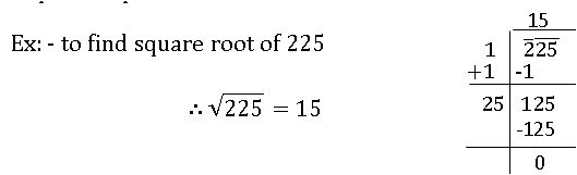
Division method: –
Steps:
- Mark off the digits in pairs starting with the unit place. Each pair and the remaining one digit are called a period.
- Think of the largest number whose square is equal to or just less than the first period. Take this number as the divisor as well as the quotient.
- Subtract the product of the divisor and quotient from the first period and bring down the next period to the right of the remainder. this becomes the new dividend.
- Now, a new divisor is obtained by taking twice the quotient and annexing with it a suitable digit which is also taken as the next digit of the quotient, chosen in such a way that the product of the new divisor and this digit is equal to or just less than the new dividend.
- Repeat steps 2, 3, and 4 till all the periods have been taken up. Thus, the obtained quotient is the required square root.
Finding the square root through subtraction of successive odd numbers:
- Subtract the first odd number (1) from a given number
- Subtract the second odd number (3) from the above result.
- Continue this process until the result will be zero (0).
- Count the steps involved above the process. No. of steps is the required answer.
Ex: find square root of 16
16 – 1 = 15; 15 – 3 = 12; 12 – 5 = 7; 7 – 7 = 0
After 4 steps we got 0.
∴ square root of 16 = 4.
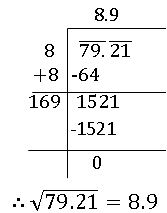
The square root of a number in decimal form
Make the no. of decimal places even, by affixing a zero, if necessary. Now periods and find out the square root by the long division method.
Put the decimal point in the square root as soon as the integral part is exhausted.
Ex: – To find the square root of 79.21
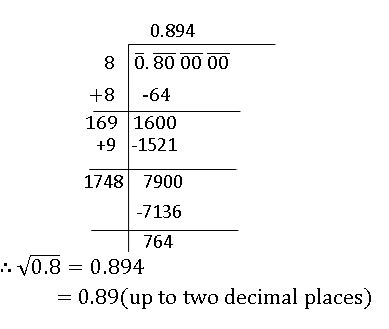
The square root of a decimal number which is not perfect square:
if the square root is required to correct up to two places of decimal, we shall find it up 3 places of decimal and then round it off up to two decimal places.
if the square root is required to correct up to three places of decimal, we shall find it up 4 places of decimal and then round it off up to three decimal places.
Ex: – To find the square root of 0.8 up to 2 decimal places
Cube of a number:
The cube of a number is that number raised to the power 3.
Ex: – cube of 0.3 = 0.33 = 0.027
Cube of 2 = 23 = 8
Perfect cube:
If a number is a perfect cube, then it can be written as the cube of some natural numbers.
Ex: – 1, 8, 27, and so on.
Cube root:
The cube root of a number x is that number which when multiplied by itself three times gives x as the product.
Cube root of x is denoted by ![]()
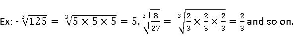
Methods of finding the cube root of given Number
Prime factorization method: –
Steps:
- Resolve the given number into prime factors.
- Make triplets of similar factors.
- The product of prime factors, choosing one out of every triplet gives the cube root of the given number.
Ex: – 27
Prim factors of 27 = 3 ×3×3
= 3
∴ cube root of 27 = 3
Estimating the cube root of a number:
Ex: estimate the cube root of 2744
Start making groups of through estimation. The first group is 744 and the second group is 2
2 744
The first group i.e., 744will give us the units digit of the cube root. As 744 ends with 4, its cube root also ends with 4. So, the unit place of cube root will be 4.
In second group number is 2
We know that 13 < 2 < 23
As the smallest number is 1, t becomes the tens place of the required cube root.
∴ cube root of 2744 = 14.
viii Class Maths
7. FREQUENCY DISTRIBUTION TABLES AND GRAPHS
Data: An information available in the numerical form or verbal form or graphical form that helps in taking decisions or drawing conclusions is called data.
Measures of central tendency:
The measures of central tendency are 3 types. They are: 1. Arithmetic mean 2. Median and 3. Mode.
1.Arithmetic Mean:
Arithmetic mean of x1, x2, x3, …. x n is ![]() ⇒
⇒ 
Where ∑xi represents the sum of all xi ’s; ‘i’ takes the values from 1 to n.
Arithmetic mean by deviation Method: –
![]()
A is assumed mean.
∎Sum of the deviations of all observations from the estimated mean is zero.
∎Arithmetic mean is a representative value of the entire data.
∎Arithmetic mean depends on both no. of observations and value of each observation in a data.
∎Arithmetic mean is unique value of data.
∎When all the observations of the data are increased or decreased by a certain number, the mean also increase or decrease by the same number.
∎When all the observations of the data are multiplied or divided by a certain number, the mean also multiplied or divided by the same number.
2.Median:
Median is the middle most value of the given data.
First, we arrange given data in ascending or descending order.
If n is the no. of observation in a data, then
Median =  observation, when n is odd.
Median =![]() when n is even.
when n is even.
∎Median is the middle most observation of the data.
∎It depends on no. of observations and middle observations of the ordered data
∎ It not effected by any change in extreme values.
3.Mode:
Mode is the most frequently occurring observation of given data.
∎Mode depends neither on no. of observations nor value of all observations.
∎It is used to analyse both numerical and verbal data.
∎ There may be two or three or many modes for the same data.
Grouped data:
If we organize the data by dividing it into convenient groups, then it is called Grouped data.
Frequency distribution or Frequency table:
The representation of classified distinct observations of the data with frequencies is called frequency distribution.
Class intervals: Small groups in a data are called Class intervals
Ex: 0 – 5, 5- 10, …
Limits and boundaries:
In the class interval 5 – 10, 5 is called the lower limit and 10 is called the upper limit.
Boundaries: The average of the upper limit of the first class and the lower limit of the second class becomes the upper boundary first class and lower boundary of the second class.
These boundaries are also called ‘true class limits’
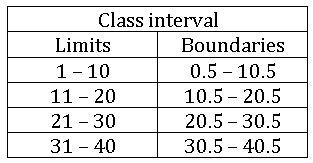
Length of the class: The difference between the upper and lower boundaries of a class is called the Length of the class.
From the above table length of the class, 0.5 – 10.5 is 10.5 – 0.5 = 10
Range: The difference between the highest and least value of given data is called a range of the data.
Construction of grouped frequency Distribution:
Ex: 1, 2, 2, 3, 3, 3, 3, 3, 4, 4, 4, 4, 4, 4, 4, 4, 4, 5, 5, 5, 5, 5, 5, 5, 6, 6, 6, 6, 7, 7
Highest value = 7; least value = 1
Range = 7 – 1 = 6.
Class interval =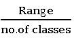
= ![]() = 0.8 approximately.
= 0.8 approximately.
Characteristics of grouped frequency distribution:
- It divides the data onto convenient and small groups called class intervals.1.
- Class intervals like 1 – 10, 11 – 20 … are called inclusive class intervals. Both the lower and upper limits of a particular class belong to that particular class.
- Class intervals like 0 – 10, 10 – 20 … are called exclusive class intervals. Only the lower limit of a particular class belongs to that class but not its upper limit.
- In exclusive class intervals, both limits and boundaries are equal.
- In inclusive class intervals, limits and boundaries are not equal.
- Individual values of all observations can not be identified from the frequency table, but the value of each observation of a particular class is assumed to be the average of the upper and lower boundaries of that class. This value is called ‘class mark’ or ‘mid value’.
Less than and greater than Cumulative frequencies:
The distribution that represents the upper boundaries of the classes and their respective less than cumulative frequencies is called ‘less than cumulative frequency distribution’
The distribution that represents lower boundaries of the classes and their respective greater than cumulative frequencies is called ‘greater than cumulative frequency distribution’
| Class intervals | frequency | LB | Greater than cumulative frequency | UB | Less than cumulative frequency |
| 0 – 5 | 7 | 0 | 36 + 7 = 43 | 5 | 7 |
| 5 – 10 | 10 | 5 | 26 + 10 = 36 | 10 | 7+10 = 17 |
| 10 – 15 | 15 | 10 | 11 + 15 = 26 | 15 | 17 + 15 = 32 |
| 15 – 20 | 8 | 15 | 3 + 8 = 11 | 20 | 32 + 8 = 40 |
| 20 – 25 | 3 | 20 | 3 | 25 | 40 + 3 = 43 |
Graphical representation of the Data:
Bar graph:
A display of information using vertical or horizontal bars of uniform width and different lengths being proportional to the respective values is called a bar graph.
Ex:
Histogram:
A graphical representation of the frequency distribution of exclusive class intervals is called a histogram.
Ex:
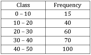
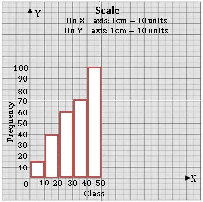
Steps on Construction:
Step-1: If class intervals are inclusive, then convert them into the exclusive form
Step-2: Choose a suitable scale on the X – axis and mark the class intervals on it.
Step-3: Choose a suitable scale on the Y – axis and mark the frequencies on it.
Scale: On X – axis 1cm = 10 units
On Y – axis 1 cm = 10 units
Step-4: Draw a rectangle with class intervals as bases and the corresponding frequencies as the corresponding heights.
Histogram with varying Base widths:
Ex:
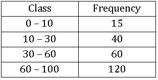
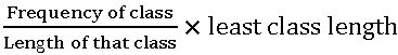
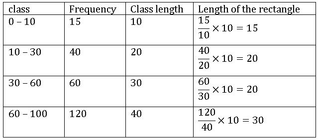
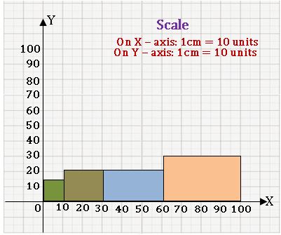
Steps on Construction:
Step-1: If class intervals are inclusive, then convert them into the exclusive form
Step-2: Choose a suitable scale on the X – axis and mark the class intervals on it.
Step-3: Choose a suitable scale on the Y – axis and mark the frequencies on it.
Scale: On X – axis 1cm = 10 units
On Y – axis 1 cm = 10 units
Step-4: Draw a rectangle with class intervals as bases and the corresponding frequencies as the corresponding heights.
Frequency polygon:
Ex:
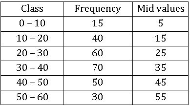
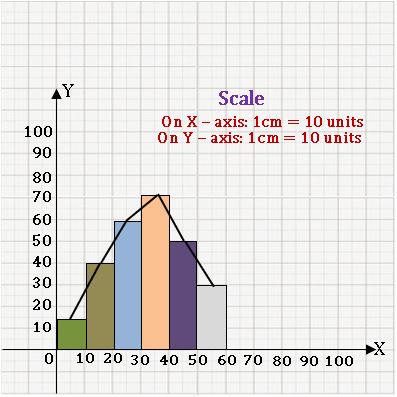
Steps on Construction:
Step-1: Calculate the midpoints of every class interval given in the data.
Step-2: Choose a suitable scale on the X – axis and mark the class intervals on it.
Step-3: Choose a suitable scale on the Y – axis and mark the frequencies on it.
Scale: On X – axis 1cm = 10 units
On Y – axis 1 cm = 10 units
Step-4: Draw the histogram for this data and mark the midpoints of the top
Step-5: Join the midpoints successfully.
Frequency curve:
Ex:
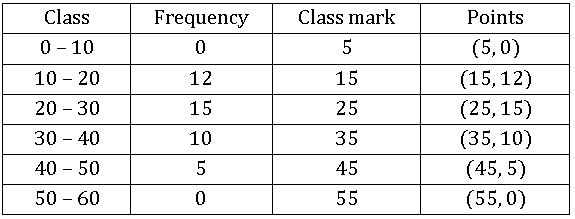
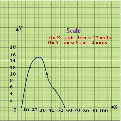
Steps on Construction:
Step-1: find the class mark of the class intervals.
Step-2: Choose a suitable scale on the X – axis and mark the class intervals on it.
Step-3: Choose a suitable scale on the Y – axis and mark the frequencies on it.
Scale: On X – axis 1cm = 10 units
On Y – axis 1 cm = 2 units
Step-4: Plot the points (which are in the above table) on the graph
Step-5: Join the consecutive points by a free-hand curve.
Less than cumulative frequency curve:
Ex:
| Class | Frequency | UB | L. C. F |
| 0 – 10 | 2 | 10 | 2 |
| 10 – 20 | 5 | 20 | 7 |
| 20 – 30 | 3 | 30 | 10 |
| 30 – 40 | 1 | 40 | 11 |
| 40 – 50 | 4 | 50 | 15 |
| 50 – 60 | 2 | 60 | 17 |
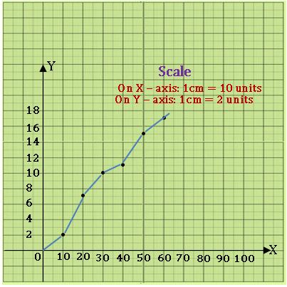
Steps on Construction:
Step-1: If class intervals are inclusive, then convert them into the exclusive form
Step-2: Construct the less-than-cumulative frequency table.
Step-3: Choose a suitable scale on the X – axis and mark the upper boundaries class intervals on it.
Choose a suitable scale on the Y – axis and mark the cumulative frequencies on it.
Scale: On X – axis 1cm = 10 units
On Y – axis 1 cm = 2 units
Step-4: If ‘x’ denotes the upper boundary of the class interval and ‘y’ denotes the corresponding cumulative frequency of a particular class, then plot (x, y) on the graph.
8.EXPLORING GEOMETRICAL FIGURES
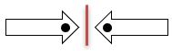
Congruent figures: The figures which have the same shape and size are called congruent figures.
Flip: Flip is a transformation in which a plane figure is reflected across a line, creating a mirror image of the original figure.
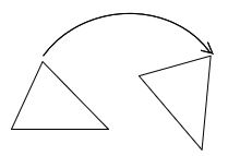
Rotation: Turning round the center is called Rotation. The distance from the center to any point on the shape stays the same. Every point makes a circular round the center.
Similar figures: The figures which have same shape but not in size are called similar figures.
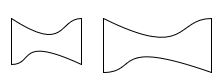
Dilation: The method of drawing enlarged or reduced similar figures is called Dilation.
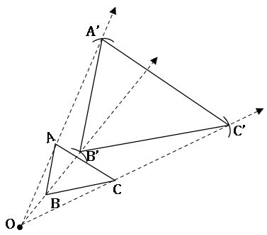
Constructing Dilation:
Ex: Construct a dilation with scale factor 3, of a triangle
Steps on Construction:
Step-1: Draw a ∆ABC and choose the centre of dilation O which is not on the triangle. Join every vertex of the triangle from O and produce
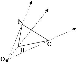
Step-2: By using compasses, mark three points A’, B’, C’ on the projection so that OA’ = 3OA; OB’ = 3OB and OC’ = 3OC.
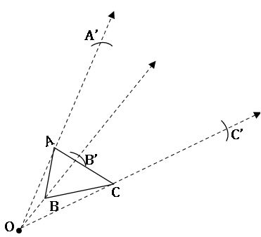
Step-3: Join A’B’, B’C’, C’A’. We observe that ∆ABC~∆A’B’C’
Symmetry:
In symmetry there are 3 types: 1. Line of symmetry, 2. Rotational symmetry and 3. Point symmetry.
1.Line of symmetry: The lines which cuts the figures exactly halves is called line of symmetry.
2.Rotational symmetry:
When an object is rotated about its centre, it comes same position after some rotation, then it is called rotational symmetry.
No. of rotations to get initial position of an object is called ‘order of position.
Ex: When a rectangle is rotated about its centre its shape resembles the initial position two times.
Order of rotation of rectangle is 2.
3.Point symmetry:
The figure looks the same either we see it from upside or it from down side is called ‘point of symmetry.
Ex: H, S, I have point of symmetry.
Tessellations: The patterns formed by repeating figures to fill a plane without gaps or overlaps are called ‘Tessellations’.
9.AREA OF PLANE FIGURES
Area of triangle:
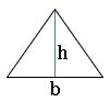
The area of triangle with base ‘b’ and height ‘h’ is ![]() square units
square units
Area of Rectangle:
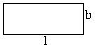
The area of rectangle with breadth ‘b’ and length ‘l’ is l × b square units.
Area of Square:

The area of triangle with side ‘a’ is a × a = a2 square units.
Area of parallelogram:
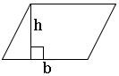
The area of the parallelogram with base ‘b’ and height ‘h’ is b × h square units.
Area of Rhombus:
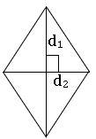
The area of Rhombus with lengths of diagonal d1, d2 is ![]() square units.
square units.
Area of Trapezium:
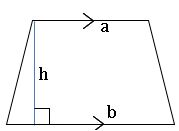
The area of the Trapezium whose lengths of parallel sides a, b and distance between the parallel side’s ‘h’ is ![]() square units.
square units.
Area of Quadrilateral:
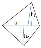
The area of Quadrilateral whose lengths of perpendiculars drawn from vertices to diagonal are h1, h2 and length of the diagonal ‘a’ is ![]() square units.
square units.
.Area of circle:
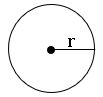
The area of circle with radius ‘r’ is π r2 square units.
Area of circular path or area of Ring:
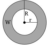
Area of ring = area of outer circle – area of inner circle
= πR 2 – π r2
= π(R 2 – r2) square units.
Length of the arc:
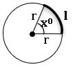
Length of the arc of a sector (l) is 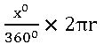
Area of sector:
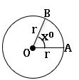
area of sector =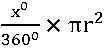
10.DIRECT AND INVERSE PROPORTIONS
Proportion: If a : b = c : d, then a, b, c and d are in proportion.
Direct proportion:
x and y are any two quantities are said to be in direct proportion, if x is increase (decrease), then y is increase (decrease).
 where k is any constant
If x1 and x2 are the values of x corresponding to the values of y1 and y2 of y respectively, then 
Inverse proportion:
x and y are any two quantities are said to be in inverse proportion, if x is increase (decrease), then y is decrease (increase).
xy = k where k is any constant
If x1 and x2 are the values of x corresponding to the values of y1 and y2 of y respectively, then 
⇒ x1y1 = x2y2.
Compound proportion:
Change in one quantity depends upon the change in two or more quantities in some proportion, then we equate the ratio of the first quantity to the compound ratio of the other two quantities.
- One quantity may be in direct proportion with the other two quantities.
- One quantity may be in inverse proportion with the other two quantities.
- One quantity may be in direct proportion with one of the two quantities and inverse proportion to with the remaining quantity.
11.ALGEBRAIC EXPRESSIONS
Term: Term is the product of constant and one or more variables.
Ex: 2x, 3xy. 5x2yz etc.
Algebraic Expression: Terms are added or subtracted to form an Algebraic Expression.
Ex; 2x + 3, 2y – 3x, 4xyz – 3x3y etc.
Monomial: If an expression contains only one term then it is called monomial.
Ex; x, 3x, – 5yz
Binomial: If an expression contains two terms, then it is called Binomial.
Ex: x + 3, x – y, 3xy – 2zx etc.
Trinomial: If an expression contains three terms, then it is called Trinomial.
Ex: x + 3 – y, x + 3xy – y, 3xy – 2z + x etc.
Like and Unlike terms: If the terms have same variable with same exponent then they are called Like terms, other wise they are called Unlike terms.
Ex: 2xy, 5yx, – 4xy are like terms
2xy, 5yz, 6zx are Unlike terms.
Addition of algebraic expressions:
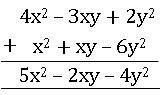
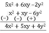
Ex: Add 4x2 – 3xy + 2y2 and x2 + xy – 6y2
Subtraction of algebraic expressions:
Ex: Subtract x2 – 2xy + 3y2 from 5x2 + 6xy – y2
Multiplication of Algebraic expressions:
For finding the product of algebraic terms we add the power of same base variables.
1.Multiplying two monomials: –
Ex: 3 × x = x + x + x = 3x.
5x × 3y = (5 × 3) × (x × y) = 15 × xy = 15xy
5x × 3x = (5 × 3) × (x × x) = 15 × x2 = 15x2(5 × 3) × (x × y) = 15 × xy = 15xy
2.Multiplying three or more monomials: –
Ex: 3 × x × y= 3xy.
5x × 3y × 4z = (5 × 3 × 4) × (x × y × z) = 60 × xyz = 60xyz
3x2 × (– 4x) × 2x3 × 2 = (3 × – 4 × 2 × 2) × (x2 × x × x3) = – 48 x6
3.Multiplying a binomial by a monomial: –
Ex: 5x (3x – 4y) = (5x × 3x) + (5x × – 4y) = 15x2 – 20xy
4.Multiplying a Trinomial by a monomial: –
Ex: 5x (3x – 4y + 4z) = (5x × 3x) + (5x × – 4y) + (5x × 4z) = 15x2 – 20xy + 20 xz
5.Multiplying a Binomial by a Binomial: –
Ex: (x + y) (2x – 3y) = x (2x – 3y) + y (2x – 3y) = 2x2 – 6 xy + 2xy – 3 y2 = 2x2 – 4xy – 3y2
6.Multiplying a Binomial by a Trinomial: –
Ex: (x + y) (2x – 3y + z) = x (2x – 3y + z) + y (2x – 3y + z)
= 2x2 – 6 xy + xz + 2xy – 3 y2 + yz
= 2x2 – 4xy – 3y2 + xz + yz
Identity: An equation is called an identity if it is satisfied by any value that replaces its variables. An equation is true for certain values for the variable in it, where as an identity is true for all its variables. There fore it is known as universally true equation.
Symbol for identity is denoted by ‘≡’ (read as identically equal to)
Some important identities:
- (a +b)2 ≡ a2 + 2ab + b2
- (a – b)2 ≡ a2 – 2ab + b2
- (a + b) (a – b) ≡ a2 – b2
- (a + b + c)2 ≡ a2 + b2 + c2 + 2ab + 2bc + 2ca
- (x + a) (x + b) ≡ x2 + (a + b) x + ab.
Geometrical verification of (a +b)2 ≡ a2 + 2ab + b2
Consider a square with side a + b
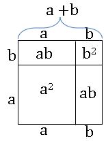
Area of square = (a + b)2
Procedure:
•Divide the square into four regions as shown in the figure.
•It consists of two squares with side ‘a’ and side ‘b’ respectively and two rectangles with length and breadth as ‘a’ and ‘b’ respectively.
•The area of given square is equal to sum of the areas of four regions.
⇒ Area of square = area of square with side a + area of square with side b + area of rectangle with sides a and b + area of the rectangle with sides and b
⇒ (a + b)2 = a2 + b2 + ab + ba
(a + b) 2 = a2 + 2ab + b2
∴ (a +b)2 ≡ a2 + 2ab + b2
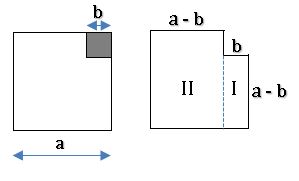
Geometrical verification of (a – b)2 ≡ a2 – 2ab + b2
Consider the square with side ‘a’
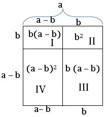
The square is divided into four regions I, II, III and IV
Area of square = area of region I + area of region II + area of region III + area of region IV
a2 = b (a – b) + b2 + b (a – b) + (a – b)2
a2 = ab – b2 + b2 + ab – b2 + (a – b)2
a2 = ab + ab – b2 + (a – b)2
⇒ (a – b)2 = a2 – ab – ab + b2
(a – b)2 = a2 – 2ab + b2
Geometrical verification of (a + b) (a – b) ≡ a2 – b2
Consider the square with side ‘a’
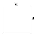
Remove the square from this whose side is ‘b’ units, we get
a2 – b2 = area of region I + area of region II
= a (a – b) + b (a – b)
= (a – b) (a + b)
∴ (a + b) (a – b) ≡ a2 – b2
12.FACFTORISATION
Factorisation:
The process of writing given expression as a product of its factors is called ‘Factorisation’.
It is helped to write the algebraic expressions in simpler form.
Irreducible factor:
A factor which can not be further expressed as product of factors is an irreducible factor.
Factorisation by Method of common factors:
Ex: Factorise 3x + 15
3x + 15 = (3 × x) + (3 ×5) (writing each term as the product of irreducible factors)
3 is the common factor of both terms
Take 3 as the common
3x + 15 = 3 × (x + 5) = 3 (x + 5)
Factorisation by grouping the terms:
Ex: Factorise ax + by + ay + bx
Firs group the like terms
ax + by + ay + bx = (ax + bx) + (ay + by)
= x (a + b) + y (a + b) (by taking out common factor from each term)
= (a + b) (x + y) (by taking out common factor from each term)
Factorisation by using identities:
- (a +b)2 ≡ a2 + 2ab + b2
- (a – b)2 ≡ a2 – 2ab + b2
- (a + b) (a – b) ≡ a2 – b2 are the algebraic identities.
Example 1:
Factorise x2 + 4x + 4
Sol: x2 + 4x + 4 = x2 + 2 (2)(x) + (2)2
It is in the form of identity (a + b)2 = a2 + 2ab + b2
x2 + 4x + 4 = (x + 2)2 = (x + 2) (x + 2).
Example 2:
Factorise x2 – 4x + 4
Sol: x2 – 4x + 4= x2 –2 (2)(x) + (2)2
It is in the form of identity (a – b)2 = a2 – 2ab + b2
x2 + 4x + 4 = = x2 –2 (2)(x) + (2)2 =(x – 2)2 = (x – 2) (x –2).
Example 3:
Factorise 4x2 – 9y2
Sol: 4x2 – 9y2 = (2x)2 – (3y)2
It is in the form of identity (a – b) (a + b) = a2 – b2
4x2 – 9y2 = (2x)2 – (3y)2 = (2x – 3y) (2x + 3y).
Factors of the form (x + a) (x + b) = x2 + (a + b) x + ab:
Ex: x2 + 12x + 35
Here we have to find out factors 35 whose sum is 12
35 = 1 × 35 1 + 35 = 36
–1 × –35 –1 –35 = –36
7 × 5 7 + 5 = 12
–7 × –5 –7 –5 = – 12
Now x2 + 12x + 35 = x2 + (7 + 5) x + 35
= x2 + 7x + 5x + 35
= x (x + 7) + 5 (x + 7)
= (x + 7) (x + 5)
Division of algebraic Expression:
1.Division of a monomial by another monomial:
Ex: 12x5 ÷ 3x
12x5 ÷ 3x =![]() =
= 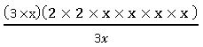
= 4x4
2.Division of an expression by a monomial:
Ex: 4x3 + 10 x2 + 8x ÷ 2x
4x3 + 10 x2 + 8x = 2 × 2 × x × x × x + 2 × 5 × x × x + 2 × 2× 2 × x
= (2x) (2x2) + (2x) (5x) + (2x) (4)
= (2x) (2x3 + 5x + 4)
4x3 + 10 x2 + 8x ÷ 2x =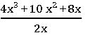
=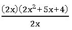
= 2x2 + 5x + 4
3.Division of an Expression by Expression:
Ex: (5x2 + 15x) ÷ (x + 3)
5x2 + 15x = 5x (x + 3)
(5x2 + 15x) ÷ (x + 3) = 
= 
= 5x
13.VISUALIZING 3-D IN 2-D
3D objects made with cubes:

Various Geometrical Solids:
Some solids (3 – D objects) have flat faces and some solids have curved faces.
Polyhedron: 3 – D objects which have flat surfaces are called polyhedron.
Ex: book, dice, cube etc.
Non – Polyhedron: 3 – D objects which have curved faces are called Non – polyhedron.
Ex: ball, pipe etc.
Faces, Edges, and Vertices of 3D – objects:
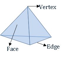
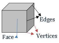
Regular polyhedron:
The polyhedron, which has congruent faces, equal edges and vertices are formed by equal no. of edges is called regular polyhedron.
Ex: Cube, Tetrahedron.
Prism: The soiled object with two parallel and congruent polygonal faces and lateral faces as rectangles or parallelograms is called a prism.
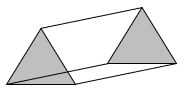
If the base of the prism is triangle, then it is called triangular prism.
If the base of the prism is square, then it is called square prism.
If the base of the prism is pentagon, then it is called pentagonal prism.
Euler’s Relation (Formula):
E + 2 = F + V
Where E = No. of edges;
F = No. of faces and
V = No. of vertices
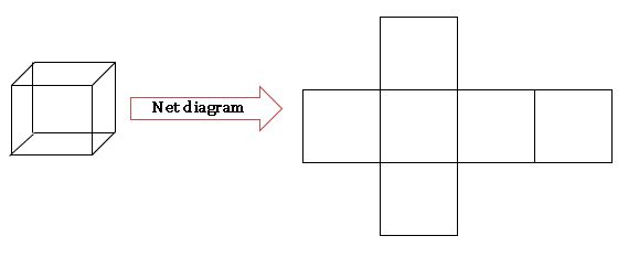
Net diagrams:
A net is a short of skeleton – outline in 2 – D, which, when folded the net results in 3 – D shape.
Ex:
Tetrahedron
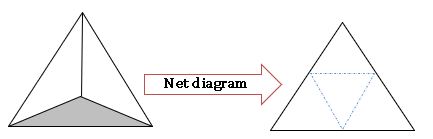
Cube
14.SURFACE AREAS AND VOLUMES
Cuboid:
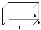
Lateral surface area (L.S.A) = 2h (l + b) square units.
Total surface area (T.S.A) = 2 (lb + bh + hl) square units.
Volume = lbh cubic units.
Cube:
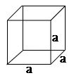
Lateral surface area (L.S.A) = 4 a2 square units.
Total surface area (T.S.A) = 6 a2 square units.
Volume = a3 cubic units.
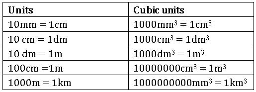
We measure volume of liquids in millilitres(ml) or litres(l)
1cm3 = 1 ml.
1000 cm3 = 1l.
1m3 = 1000000cm3 = 1000 l. = 1 kl. (kilo litre).
TS 8th Class Maths Concept
15.PLAYING WITH NUMBERS
Divisibility:
If a number ‘a’ divides another number ‘b’ completely, then ‘b’ is divisible by ‘a’.
Place value of digit:

Place value of 7 is 7 000000.
Place value of 6 is 6000
Place value of 3 is 30
Divisibility Rules:
Divisibility rule by 2: –
If the unit place of a given number is 0, 2, 4, 6, 8 then that number is divisible by 2.
Ex: 10, 12, 526 etc.
Divisibility rule by 3: –
If the sum of the digits of a given number is divisible by 3, then that number is divisible by 3.
Ex: 234
Sum of the digits = 2 + 3 + 4 = 9
9 is divisible 3
∴ 234 is divisible by 3
Divisibility rule by 4: –
If the last two digits of a given number is divisible by 4, then that number is divisible by 4.
Ex: 324
24 is divisible by 4
∴ 324 is divisible by 4
∴ 324 is divisible by 4
Divisibility rule by 5: –
If the units place of given number is 0 or 5, then it is divisible by 5.
Ex: 10, 15, 235, 480 etc.
Divisibility rule by 6: –
If a number is divisible by both 3 and 2 then that number is divisible by 6.
Ex: 324
324 is divisible by both 3 and 2
∴ 324 is divisible by 6
Divisibility rule by 7: –
Fist multiply the last digit of given number by 2,
subtract this result from the number formed by remaining digits of given number.
If that result is divisible by 7, then the given number is divisible by 7.
Ex: 112
Last digit is 2 ⇒ 2 × 2 = 4
Now 11 – 4 = 7
7 is divisible by 7
∴ 112 is divisible by 7.
Divisibility by 8: –
if the last three digits of a number is divisible by 8, then that number is divisible by 8.
Ex: – 4232, last three digits 232 are divisible by 8
∴ 4232 is divisible by 8.
Divisibility by 9: –
if the sum of the digits of a number is divisible by 9, then that number is divisible by 9.
Ex: – 459, 4 + 5 + 9 = 18 → 18 is divisible by 9 ∴ 459 is divisible by 9
532, 5 + 3 + 2 = 10 → 10 is not divisible by 9 ∴ 532 is not divisible by 9.
Divisibility by 10: –
a number is divisible by 10, if its once place is 0.
Ex: – 20 is divisible by 10. 22, 45 are not divisible by 10.
Divisibility by 11: –
A number is divisible by 11, if the difference between the sum of the digits at odd places and the sum of the digits at even places is either 0 or 11.
Ex: – 6545
Sum of the digits at odd places = 5 + 5 = 10
Sum of the digits at even places = 4 + 6 = 10
Now difference is 10 – 10 = 0
∴ 6545 is divisible by 11.
- TS 6th Maths Concept
- TS 7th Maths Concept
- TS 8th Maths Concept
- TS 9th Maths Concept
- TS 10th Maths Concept
TS 8th Class Maths Concept
Visit my Youtube Channel: Click on Below Logo